Data Preprocessing(数据预处理)
以下内容来自Udemy上的课程: Machine Learing A-Z: Hands-On Python & R in Data Science.
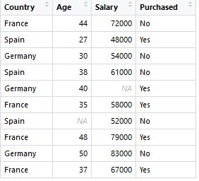
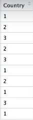
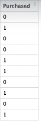
使用数据:
1. Missing data
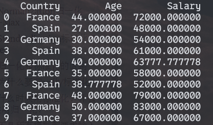
Common strategy: replace the missing data by the mean, median, or most frequent value of the feature column.
Python
1.以均值代替:
1 | # Importing the libraries |
2.以指定值替代
例:现有 df_age 如下:
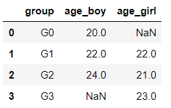
Fill the missing data in column "age_boy" with 22 and fill the missing data in column "age_girl" with 21. The expected output is:
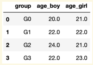
1 | df_age = df_age.fillna(value={'age_boy':22,'age_girl':21}) |
关于fillna:
1 | DataFrame.fillna(value=None, *, method=None, axis=None, inplace=False, limit=None, downcast=<no_default>) |
3.删掉有缺失值的行
1 | X.dropna(axis = 0, inplace = True) |
4.删掉有缺失值的列
1 | X.dropna(axis = 1, inplace = True) |
R
1 | # Importing the dataset |
2. Categorical data
Python
1 | # 使用上一步处理缺失值后的数据 |
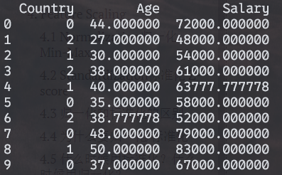
X:
2.1 LabelEncoder
LabelEncoder官方文档
https://scikit-learn.org/dev/modules/generated/sklearn.preprocessing.LabelEncoder.html
1.使用LabelEncoder对X编码
1 | from sklearn.preprocessing import LabelEncoder |
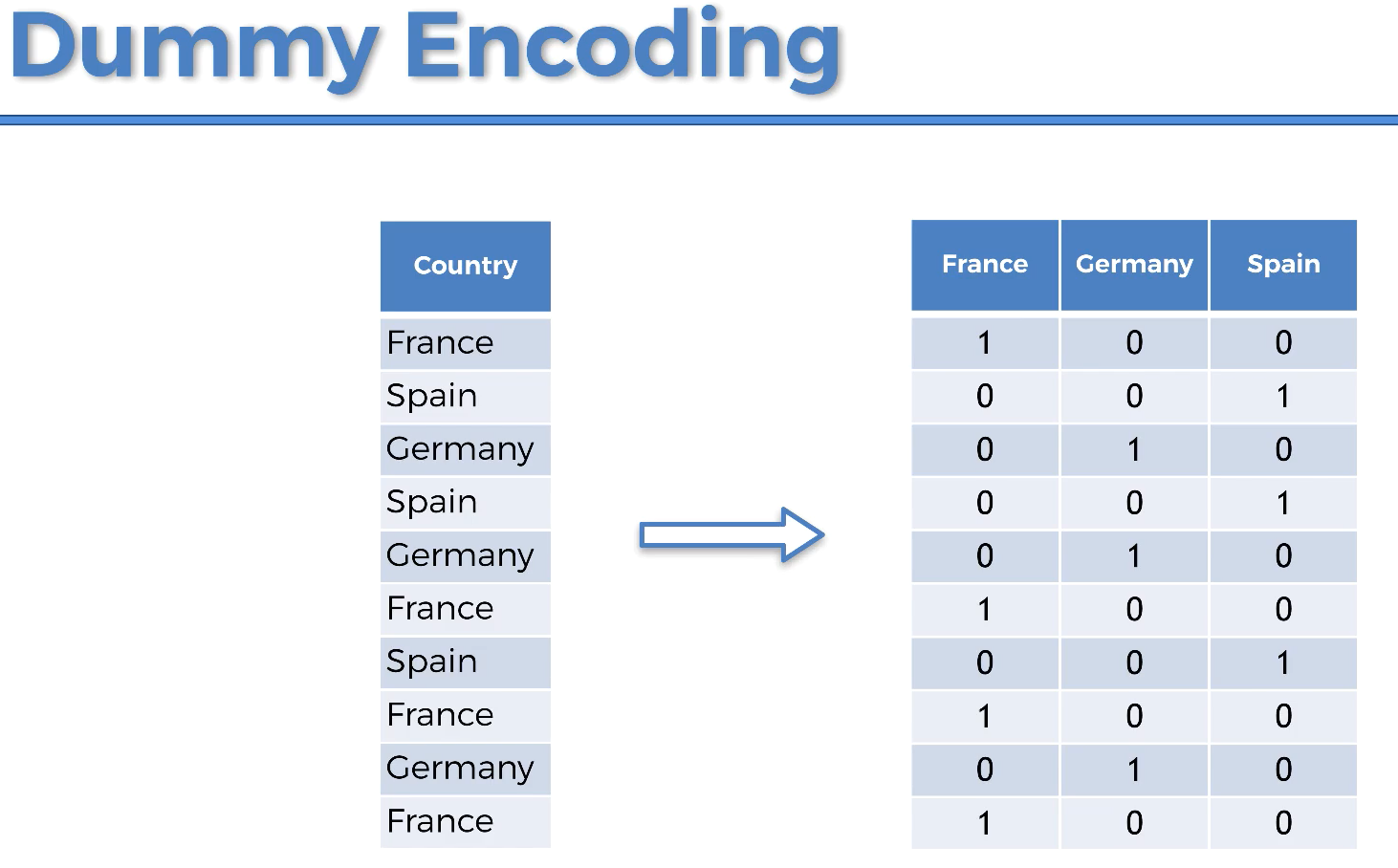
经过LabelEncoder编码后的X:
But the model will think that France has lower value than Spain -> that's not the case, we have no order here. 解决办法:使用后面介绍的OneHotEncoder方法。(如果是S, M, L of a T-shirt(本身有顺序), 不必使用OneHotEncoder方法。)
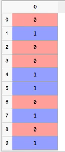
2.使用LabelEncoder对y编码
1 | # Encoding the Dependent Variable |
2.2 factorize
1 | import pandas as pd |
比较与LabelEnocoder的结果:
1 | # LabelEncoder |
👆可以看到factorize与LabelEncoder结果是一样的
2.3 OneHotEncoder
OneHotEncoder官方文档
https://scikit-learn.org/stable/modules/generated/sklearn.preprocessing.OneHotEncoder.html
1 | from sklearn.preprocessing import OneHotEncoder |
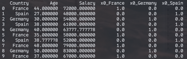
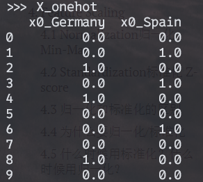
X_new: (再把第一列drop掉)
上述结果,还应该drop掉France, Germany, Spain的其中一列(只需要两列就够了),更好的写法:
1 | onehotencoder=OneHotEncoder(drop='first') |
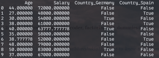
2.4 get_dummies
onehot encoding的另一种实现方法
1 | X = pd.get_dummies(X, drop_first=True) |
2.4 LabelEncoder, OnehotEncoder, factorize, get_dummies的区别
参考
https://medium.com/@vaibhavshukla182/want-to-know-the-diff-among-pd-factorize-a8591eb3347d
这四种编码方式可以分为两类:
- Encode labels into categorical variables: Pandas
factorizeand scikit-learnLabelEncoder. 编码结果是1维的. factorize与LabelEncoder都是将字符型变量(categorical varirables)编码为数值型1,2,3...(本来是一维,编码后依然是一维) - Encode categorical variable into dummy/indicator (binary)
variables: Pandas
get_dummiesand scikit-learnOneHotEncoder. 编码结果是 n 维的. get_dummies与OneHotEnocder都是将字符型变量编码为0,1哑变量(本来是一维,编码后变为多维)
The main difference between pandas and scikit-learn encoders is that
scikit-learn encoders are made to be used in scikit-learn
pipelines with fit and transform
methods. sklearn中的LabelEnocder,OneHotEncoder与pandas中的factorize,
get_dummies的区别在于sklearn的两个方法可以使用fit和transform(在测试集上的编码应依赖于训练集)
R
1 | # Encoding categorical data |
3. train_test_split
Python
1 | # Importing the dataset |
R
1 | # Importing the dataset |
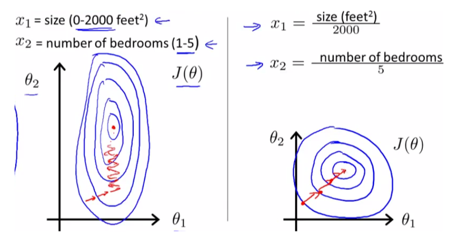
4. Feature Scaling
Lots of machine learning models are based on Euclidean distance. Since the salary has a much wider range of values, the euclidean distance will be dominated by the salary.
Even if the machine learning models are not based on euclidean distance, we will still need to do feature scaling, because the algorithms will converge much faster.
Feature Scaling: Putting our variables in the same range (in the same scale), so that no variable is dominated by the other.
Question 1: Do we need to fit and transform dummy variables?
It depends on the context. Depends on how much you want to keep interpretation in your models. Because if we scale dummy variables, it will be good because everything will be on the same scale, it will be good for our predictions, but we will lose interpretation of knowing which observation belongs to which country.
Qustion 2: Do we need to apply feature scaling to y?
we don't need to do it if it is a classification problem with categorical dependent variable. But for regression, where the dependent variable will take a huge range of values, we will need to apply feature scaling to y as well.
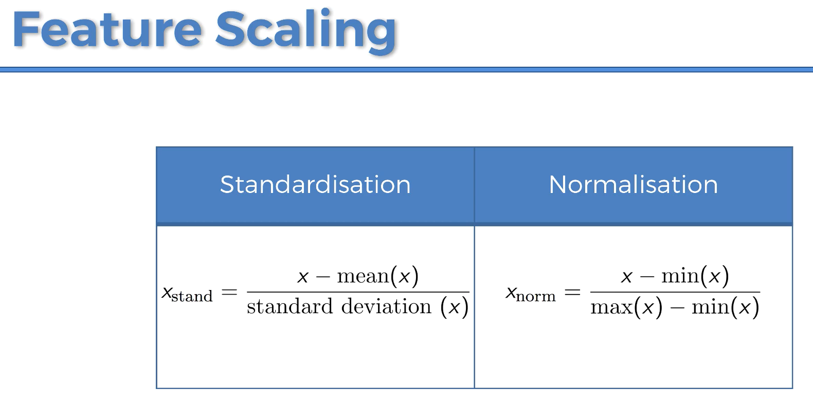
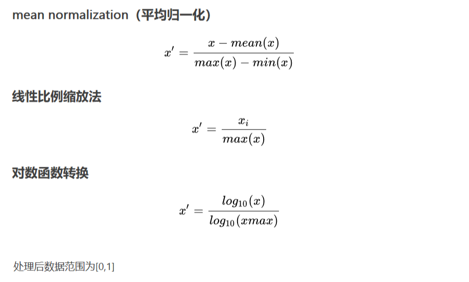
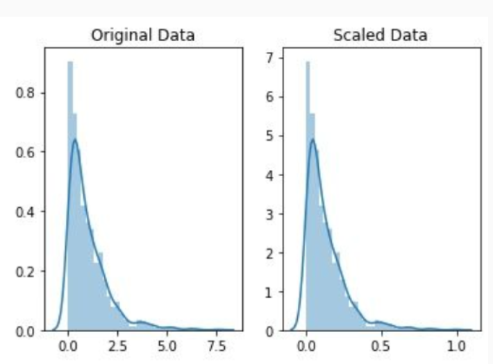
4.1 Normalization归一化 Min-Max
\[ x_{new} = \frac{x_{old}-x_{min}}{x_{max}-x_{min}} \]
\(x_{new}\)取值范围:[0,1]
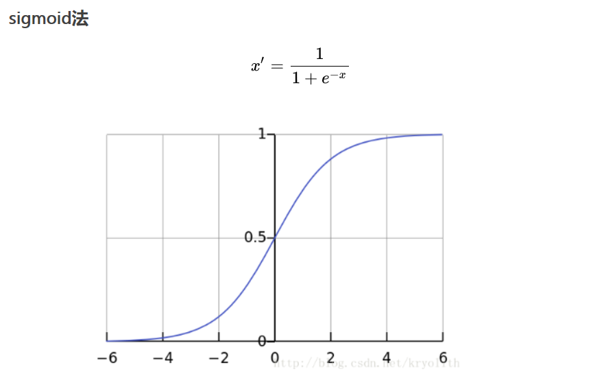
其他归一化方法:
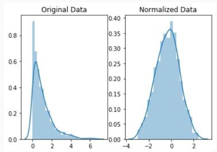
4.2 Standardization标准化 Z-score
\[ x_{new} = \frac{X_{old}-\mu}{\sigma} \]
The resulting values hover around 0, and typically range between -3 and +3, but can be higher or lower.
4.3 归一化和标准化的区别
(1)转换区间 归一化(Normalization):把数据转换到(0,1)或者(-1,1)区间的数据映射方式 标准化(Standardization):把数据转换到均值为0,标准差为1的数据映射方式
(2)数据分布 归一化:对数据的数值范围进行特定缩放,但不改变其数据分布
标准化:对数据的分布进行转换,使其符合某种分布(如正态分布)
4.4 为什么要归一化/标准化
(1)梯度下降的需要,加速算法收敛速度 在使用梯度下降的方法求解最优化问题时,归一化/标准化后可以加快梯度下降的求解速度,即提升模型的收敛速度。
线性回归、逻辑回归、神经网络等使用梯度下降法求解最优参数的算法,输入数据需要做归一化/标准化处理,提升模型收敛速度。
(2)距离计算的需要,保障算法准确度 一些算法需要计算样本之间的距离(如欧式距离),例如KNN、kmeans等聚类算法。如果一个特征值域范围非常大,那么距离计算就主要取决于这个特征,从而与实际情况相悖。
(3)消除量纲和数量级影响 各个指标之间由于计量单位和数量级不尽相同,从而使得各指标间不具有综合性,不能直接进行综合分析,这时就必须采用某种方法对各指标数值进行无量纲化处理,解决各指标数值不可综合性问题。
去量纲指的是去除数据单位之间的不统一,将数据统一变换为无单位(统一单位)的数据集。
4.5 什么时候用标准化?什么时候用归一化?
(1)一般建议优先使用标准化,在机器学习中,标准化是更常用的手段,归一化的应用场景是有限的。 (2)如果数据不稳定,存在极端的最大最小值,不要用归一化。 (3)在分类、聚类算法中,需要使用距离来度量相似性的时候、或者使用PCA技术进行降维的时候,标准化(Z-score standardization)表现更好。 (4)在不涉及距离度量、协方差计算、数据不符合正态分布的时候,可以使用归一化方法。比如图像处理中,将RGB图像转换为灰度图像后将其值限定在[0, 255]的范围。
4.6 不是所有模型都要求输入数据经过标准化/归一化处理
不是所有的模型都需要做归一的,比如模型算法里面没有关于对距离的衡量,没有关于对变量间标准差的衡量。 (1)比如decision tree决策树,算法里面没有涉及到任何和距离等有关的,所以在做决策树模型时,通常是不需要将变量做标准化的 (2)概率模型不需要归一化,因为它们不关心变量的值,而是关心变量的分布和变量之间的条件概率。
4.7 Python
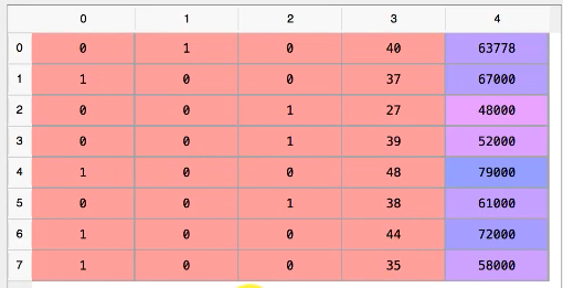
标准化:(假设数据已经过缺失值处理与categorical data的转换)
(以下代码中scale了dummy variable.)
1 | # Importing the dataset |
Feature scaling on X_test is the same as the feature scaling on the X_train(scaled on the same bases)
The result is between -1 and 1.
1 | sc_y = StandardScaler() |
归一化MinMax:
1 | from sklearn.preprocessing import MinMaxScaler |
4.8 R
1 | # Splitting the dataset into the Training set and Test set |
语法:scale(x, center = TRUE, scale = TRUE)
Arguments: x: a numeric matrix(like object).
center: either a logical value or a numeric vector of
length equal to the number of columns of x.
scale: either a logical value or a numeric vector of length
equal to the number of columns of x.
Details: If center is TRUE then centering
is done by subtracting the column means (omitting NAs) of
x from their corresponding columns, and if
center is FALSE, no centering is done. If
scale is TRUE then scaling is done by dividing
the (centered) columns of x by their standard deviations if
center is TRUE, and the root mean square
otherwise. If scale is FALSE, no scaling is
done. The root-mean-square for a (possibly centered) column is defined
as \(\sqrt{sum(x^2)/(n-1)}\), where
x is a vector of the non-missing values and n is the
number of non-missing values. In the case center = TRUE,
this is the same as the standard deviation, but in general it is not.
(To scale by the standard deviations without centering, use
scale(x, center = FALSE, scale = apply(x, 2, sd, na.rm = TRUE)).)
但直接这样运行会出错:
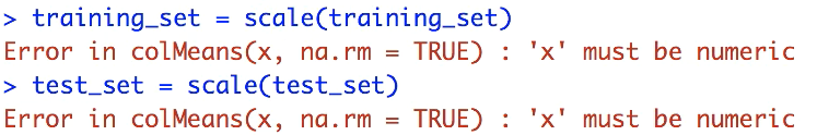
原因:因子型变量不是 numeric的。
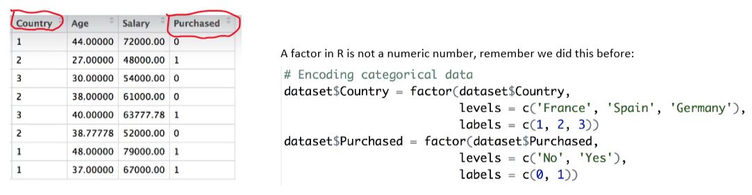
解决方法:We're going to exclude categories from the feature scaling, we're not going to apply feature scaling on those columns.
1 | training_set[,2:3] = scale(training_set[,2:3]) |