Neighborhood-Based Collaborative Filtering 协同过滤
This is the idea of leveraging the behavior of others to inform what you might enjoy. At a very high level, it means finding other people like you and recommending stuff they liked. Or it might mean finding other things similar to the thing that you like.
That's why we call it collaborative filtering. It's recommending stuff based on other people's collaborative behavior.
The heart of neighborhood-based collaborative filtering is the ability to find people similar to you, or items similar to items you've liked.
1. Measuring Similarity, and Sparsity
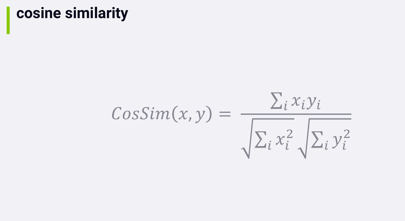
这里的余弦相似度和前面content-based中的余弦相似度的区别在于:Our dimensions would be things like his: Did this user like this thing? Or was this thing liked by this user? So every user or every thing might constitute its own dimension, and the dimensions are based on user behavior instead of content attributes.
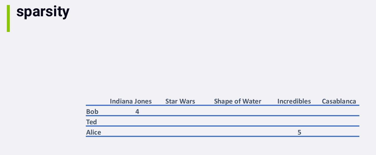
The big challenge in measuring these similarities based on behavior data is the sparsity of the data we're working with. This means that it's tough for collaborative filtering to work well unless you have a lot of user behavior data to work with. You can't compute a meaningful cosine similarity between two people when they have nothing in common, or between two items when they have no people in common.
This is why collaborative filtering works well for big companies like Amazon and Netflix. They have millions of users and so they have enough data to generate meaningful relations in spite of the data sparsity.
Sparsity also introduces some computational challenges. You don't want to waste time storing and processing all of that missing data, so under the hood we end up using structures like sparse arrays that avoid storing all that empty spaces in this matrix.
2. Similarity Metrics
Adjusted Cosine
It's applicable mostly to measuring the similarity between users based on their ratings. It's based on the idea that different people might have different baselines. What Bob considers a three star movie, maybe different from what Alice considers a three star movie.
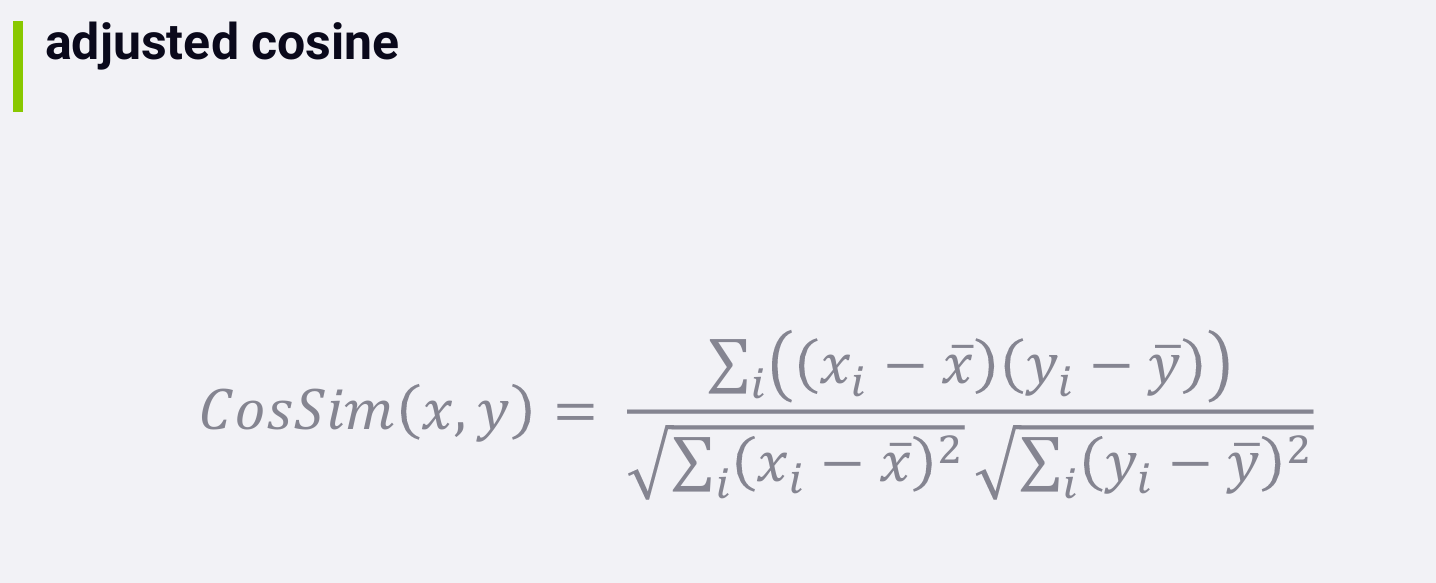
Adjusted cosine attempts to normalize these differences. Instead of measuring similarities between people based on their raw rating values, we instead measure similarities based on the difference between a user's rating for an item and their average rating for all items.
Now this sounds good on paper, but in practice, data sparsity can really mess you up here. You can only get a meaningful average, or a baseline of an individual's ratings if they have rated a lot of stuff for you to take the average of in the first place. 若有许多用户只评价了一部电影,then that data will be totally wasted with the adjusted cosine metric. 不管他们评了多少分,the difference between it and that user's mean will be zero at that point.
So, adjusted cosine might be worth experimenting with, but only if you know that most of your users have rated a lot of stuff implicitly or explicitly. And if you have that much data to begin with, these differences between individuals will start to work themselves out anyway. So, you're not likely to see as much of a difference as you might expect when using adjusted cosine.
(item-based) pearson similarity
与adjusted cosine的区别在于, we look at the difference between rating and the average from all users for that given item.
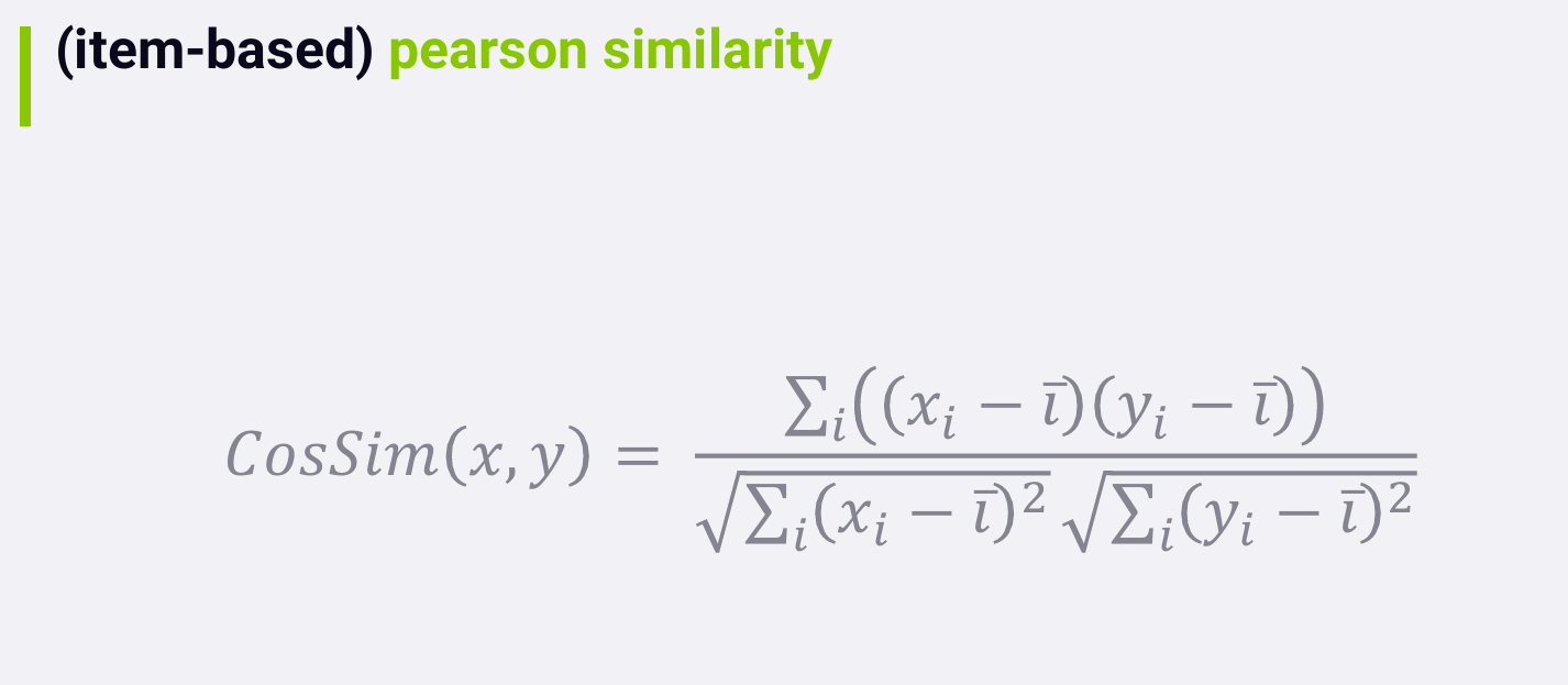
You can think of pearson similarity as measuring the similarity between people by how much they diverge from the average person's behavior. 例如,假设大多数人都喜欢Star Wars, people who hate Star Wars are going to get a very strong similarity score from pearson similarity, because they share opinions that are not mainstream.
Note that the only difference between this and adjusted cosine is whether we're talking about users or items. 这门课使用的suprise library, refers to adjusted cosine as user-based pearson similarity, because it's basically the same thing.
spearman rank correlation
- Instead of using an average rating value for a movie, 我们使用 its rank amongst all movies based on their average rating.
- Instead of individual ratings for a movie, we'd rank that movie amongst all that individual's ratings.
Spearman的主要优势在于 it can deal with ordinal data effectively. 例如,if you had a rating scale, where the difference in meaning between different rating values were not the same. I've never seen this actually used in real world applications, but you may encounter it in the academic literature.
mean squared difference
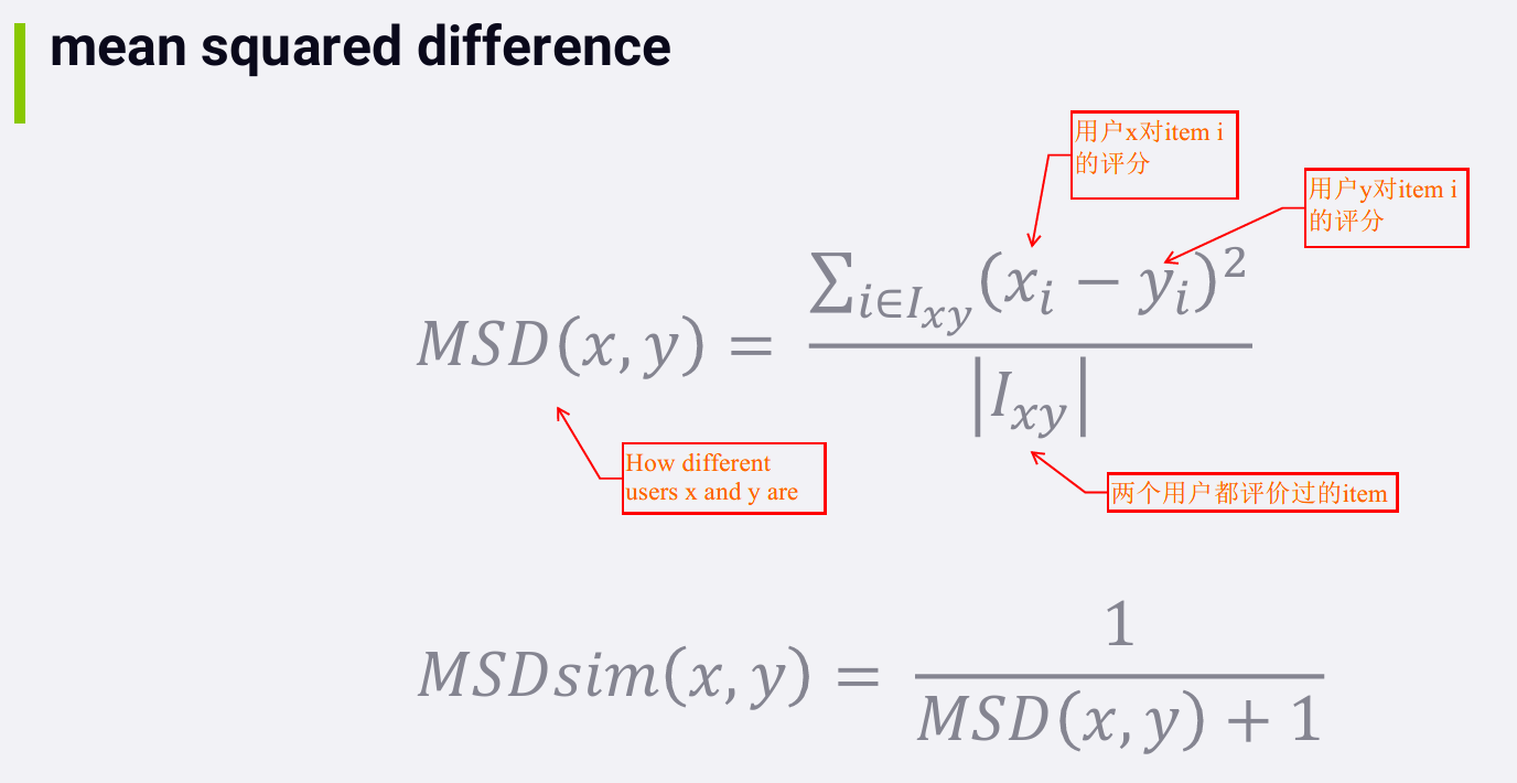
另一方面,我们可以将它应用到item上:x和y指两个不同的item, and then we'd be looking at the differences in ratings from the people these items have in common (所有评价过这两个item的人对这两个item评分的差异).
There are two ways of doing collaborative filtering, item based and user based, and it's important to remember that most of these similarity metrics can apply to either approach.
MSD 要比余弦相似度更好理解, 但 in practice, 你通常会发现cosine works better.
jaccard similarity
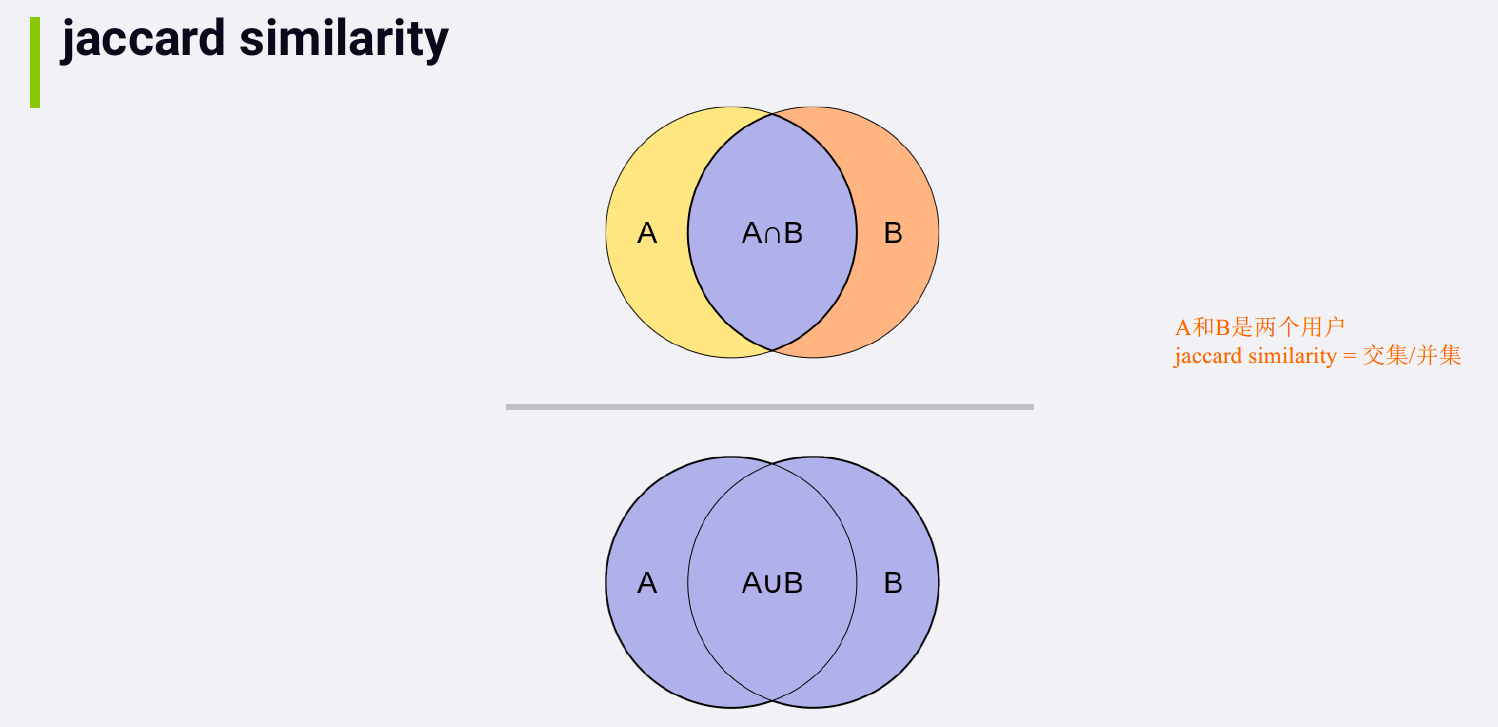
jaccard similarity 没有使用实际的rating vlaue. If you are dealing with implicit ratings, for example, just the fact that somebody watched something, in this case, Jaccard can be a reasonable choice that's very fast to compute.
Recap

- Cosine similarity is almost always a reasonable thing to start with.
- Adjust cosine and Pearson are two different terms for basically the same thing. It's mean centered cosine similarities. The idea is to deal with unusual rating behavior that deviates from the mean, but in practice, it can sometimes do more harm than good.
- Spearman ranking correlation is the same idea as Pearson, using ranking instead of raw ratings, and it's not something you are likely to be using in practice.
- MSD is mean squared difference, which is just an easier similarity metric to warp your head around than cosine similarity, but in practice, it usually doesn't perform better.
- Jaccard similarity is just looking at how many items two users have in common, or how many users two items have in common, divided by how many items or users they have between both of them. It's really simple and well suited to implicit ratings, like binary actions, like purchasing or view something. But you can also apply cosine similarities to implicit ratings too.
- So, and the end of the day, cosine similarity remains my default go to similarity metric.
3. 协同过滤
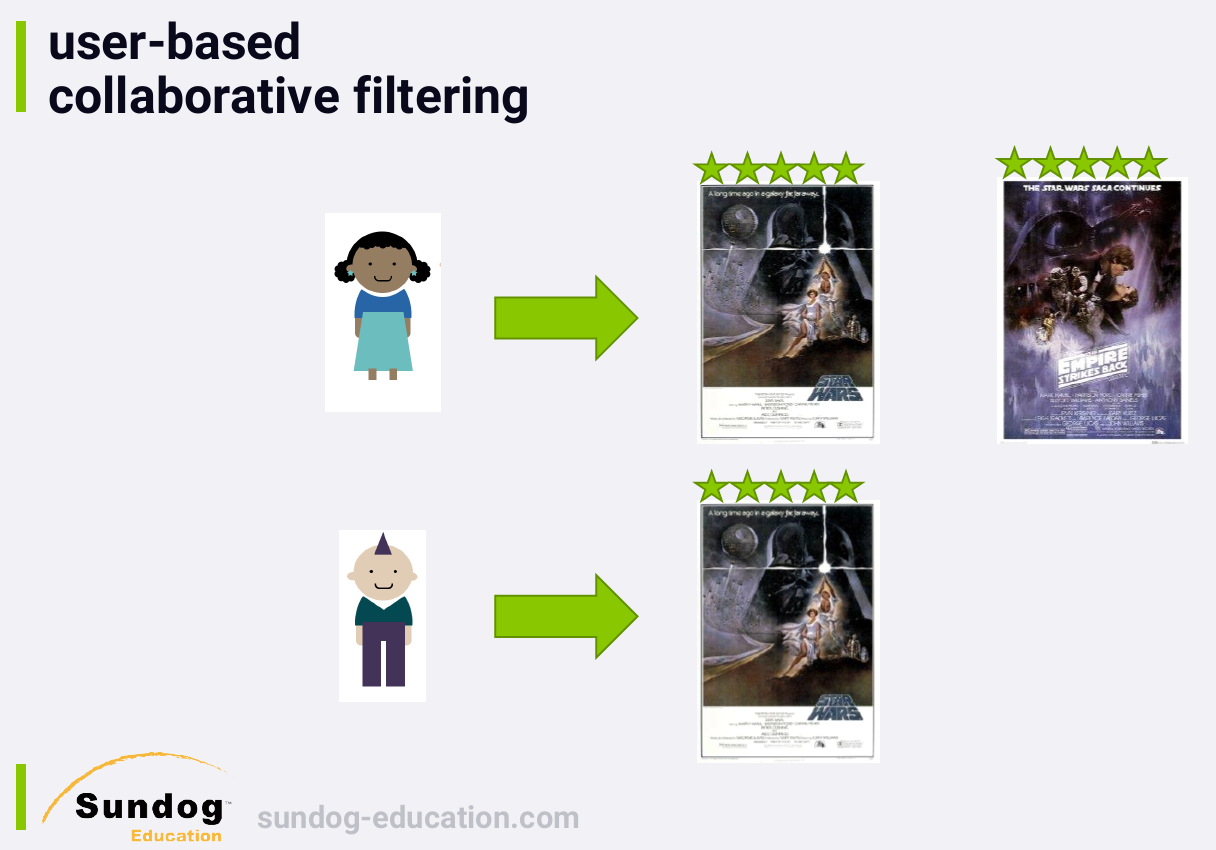
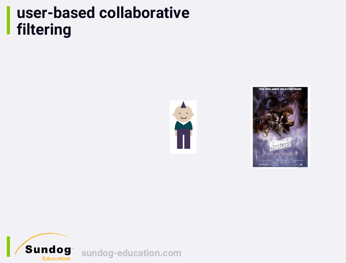
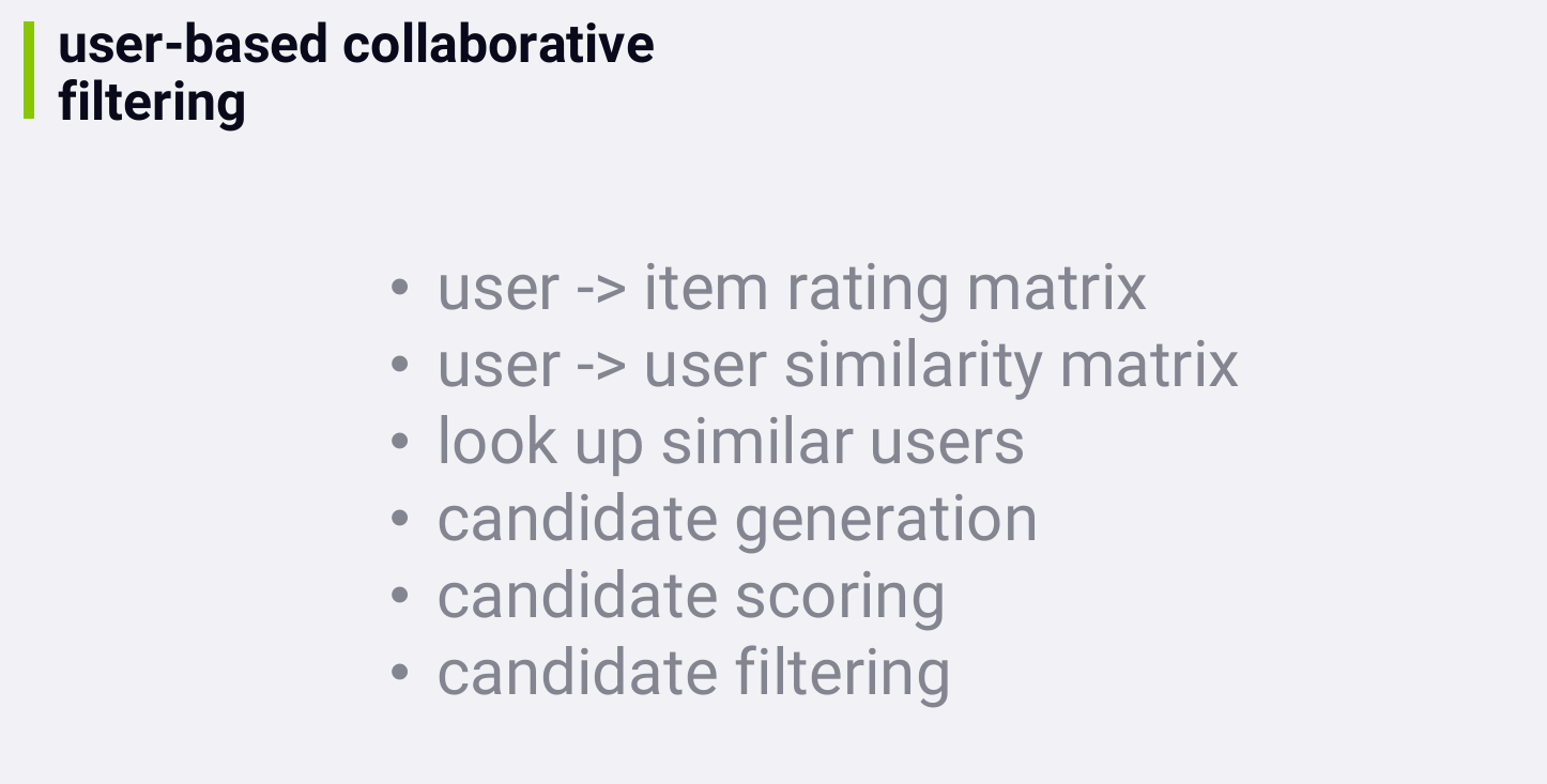
3.1 User-based Collaborative Filtering 基于用户的协同过滤(UserCF)
与基于物品的协同过滤类似的,不同的是,基于物品的协同过滤的原理是用户 U 购买了 A 物品,推荐给用户 U 和 A 相似的物品 B、C、D。而基于用户的协同过滤,是先计算用户 U 与其他的用户的相似度,然后取和 U 最相似的几个用户,把他们购买过的物品推荐给用户U。
3.1.1 计算用户之间的相似度
参考 https://github.com/NLP-LOVE/ML-NLP/tree/master/Project/17.%20Recommendation%20System
为了计算用户相似度,我们首先要把用户购买过物品的索引数据转化成物品被用户购买过的索引数据,即物品的倒排索引:
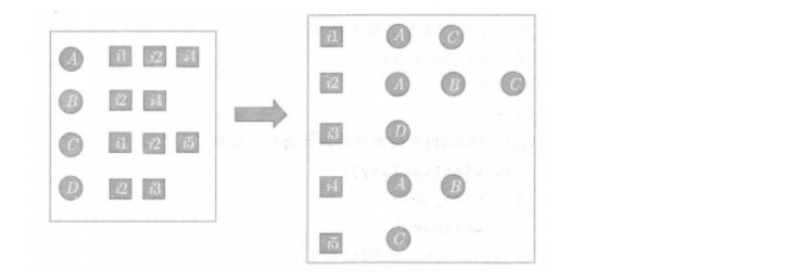
建立好物品的倒排索引后,就可以根据相似度公式计算用户之间的相似度:
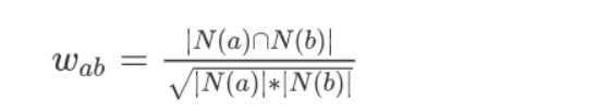
其中 \(N(a)\) 表示用户 \(a\) 购买物品的数量,\(N(b)\) 表示用户 \(b\) 购买物品的数量,\(N(a)∩N(b)\) 表示用户 \(a\) 和 \(b\) 购买相同物品的数量。有了用户的相似数据,针对用户 U 挑选 k 个最相似的用户,把他们购买过的物品中,U 未购买过的物品推荐给用户 U 即可。
3.1.2 举例
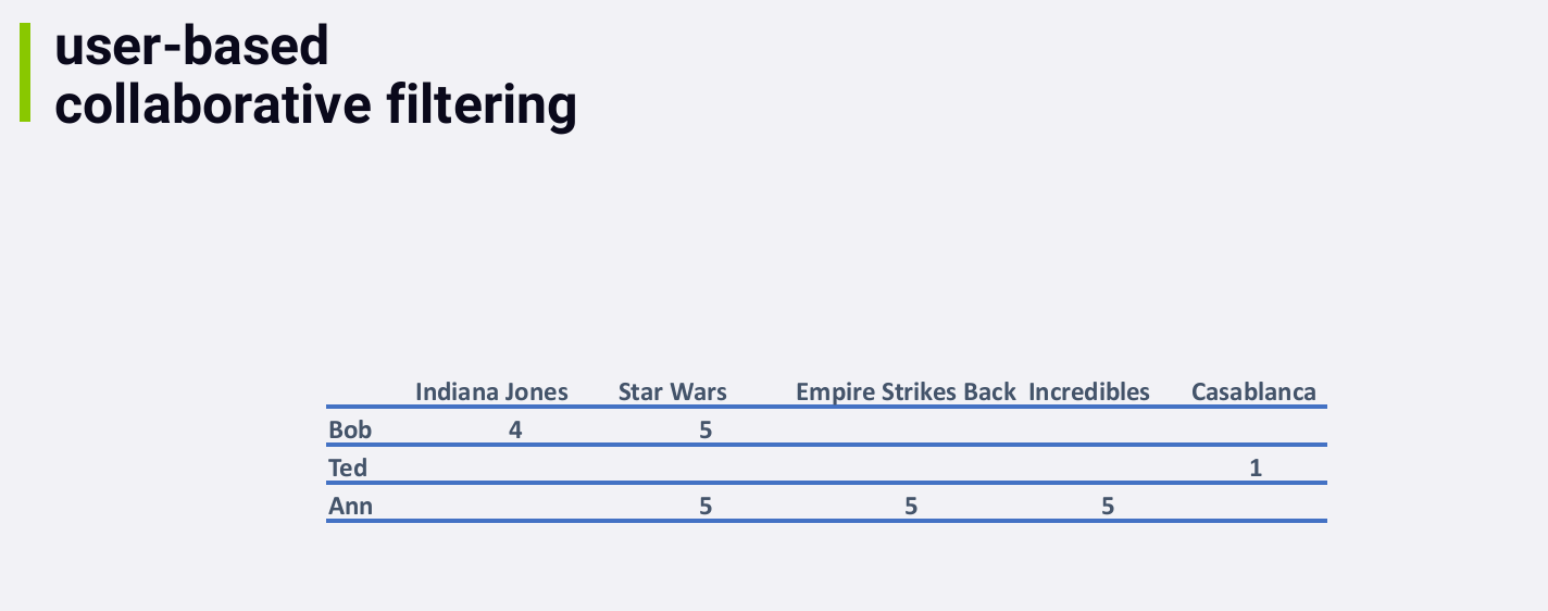
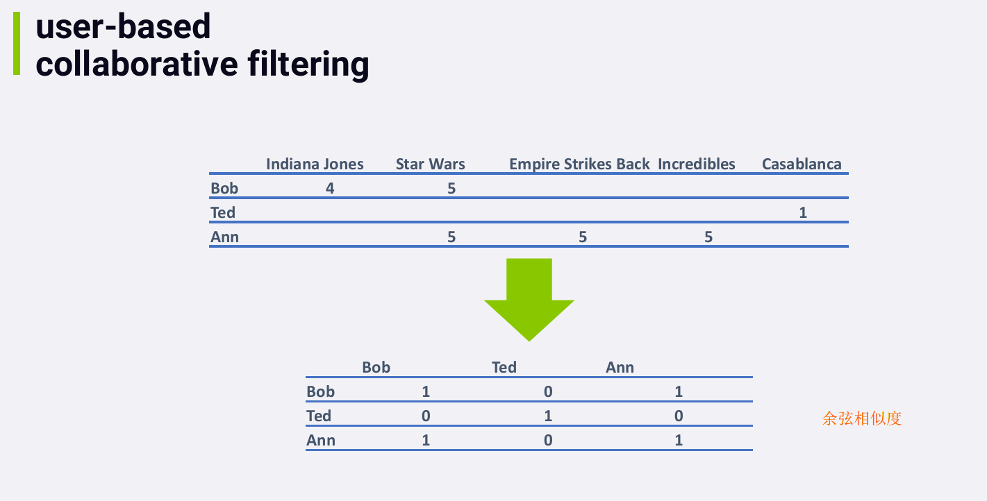
- 每个人和自己的余弦相似度是1
- Bob 和 Ted的余弦相似度是0,因为他们没有评价过相同的电影
- 矩阵的上三角部分和下三角部分是对称的
- 对于 Bob 和 Ann, 虽然他们评价过不同的电影,当我们考虑相似度时,我们只看他们共同评价过的电影。在这个例子中,他们共同评价过的电影只有一部,并且评分都为5,所以他们的相似度得分为1 (100%)。
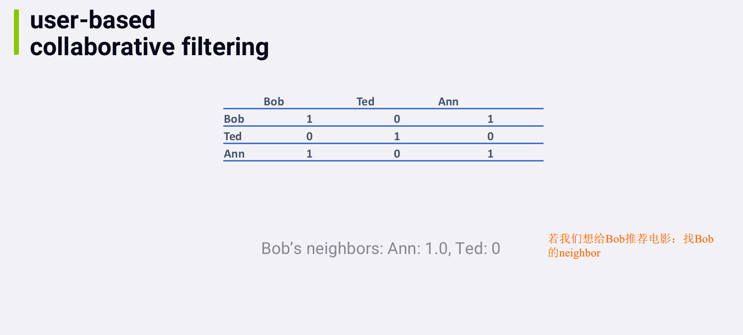
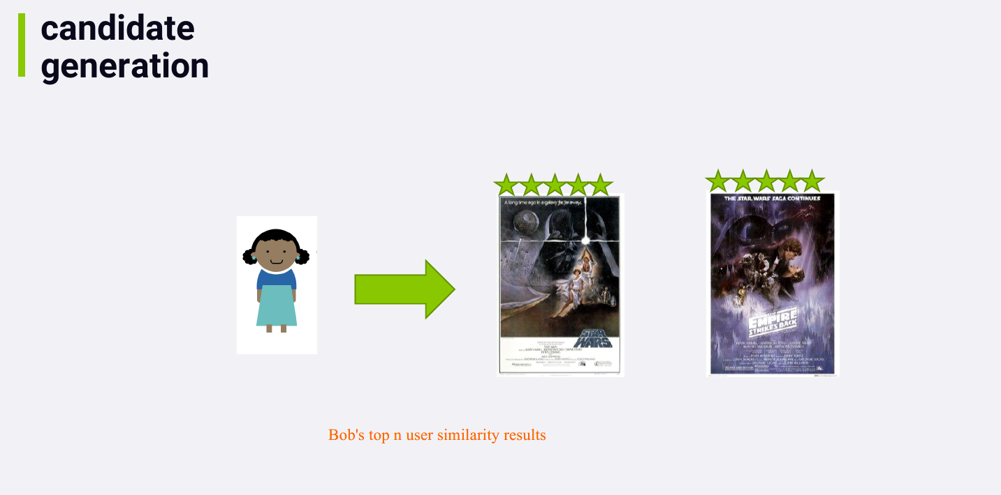
注:两个用户的相似度为100%并不一定代表他们喜欢相同的东西,也可以代表他们都讨厌相同的东西(例如,若 Bob 和 Ann 都给Star Wars打1分,他们仍然是100% similar)。事实上,the math behind cosine similarity works out such that if you only have one movie in common, you end up with 100% similarity no matter what. Even if Bob loved Star Wars and Ann hated it, in a sparse data situation, they both end up 100% similar. Sparse data is a huge problem with collaborative filtering, and it can lead to weird results. And sometimes, you need to enforce a minimum threshold on how many movies users have in common before you consider them at all.
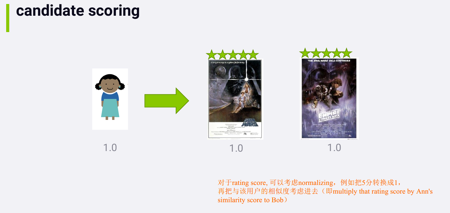
除了normalizing, 还可以例如将评分为1、2的转换成negative score, 方法不唯一,没有标准的方法,可通过试验看 what works best for the data you have.
应该adding in the score for a given movie if we encounter it more than once.
3.1.3 Recap
3.1.4 User-based Collaborative Filtering, Hands-On
code walkthrough
CollaborativeFiltering文件夹里的:
运行SimpleUserCF.py
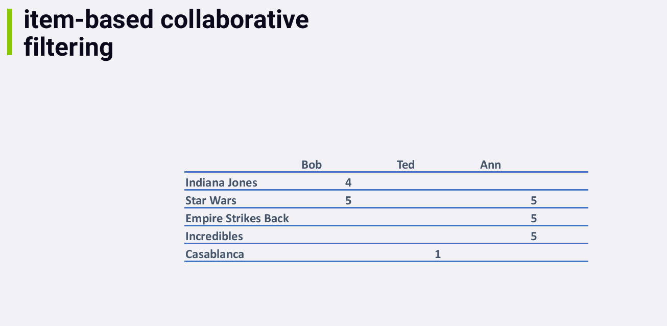
3.2 Item-based Collaborative Filtering 基于物品的协同过滤(ItemCF)
Look at the things you liked, and recommend stuff that's similar to those things.
核心思想:给用户推荐那些和他们之前喜欢的物品相似的物品。

一些原因为什么使用物品之间的相似度可能比使用用户之间的相似度更好:
- Items tend to be of a more permanent nature than people. An individual's test may change very quickly over the span of their lives. Your math book will always be similar to other math books. As such, you can get away with computing an item similarity matrix less often than user similarities, because it won't change very quickly.
- You usually have far fewer items to deal with than people. There are way more people than there are things to recommend to them in most cases. 即物品相似度矩阵会比用户相似度矩阵会小很多,这样不仅 make it simpler to store that matrix, it makes faster to compute as well. And when you're dealing with massive systems like Amazon and Netflix, computational efficiency is very important. Not only does it require fewer resources, it means you can regenerate your similarities between items more often, making your system more responsive when new items are introduced.
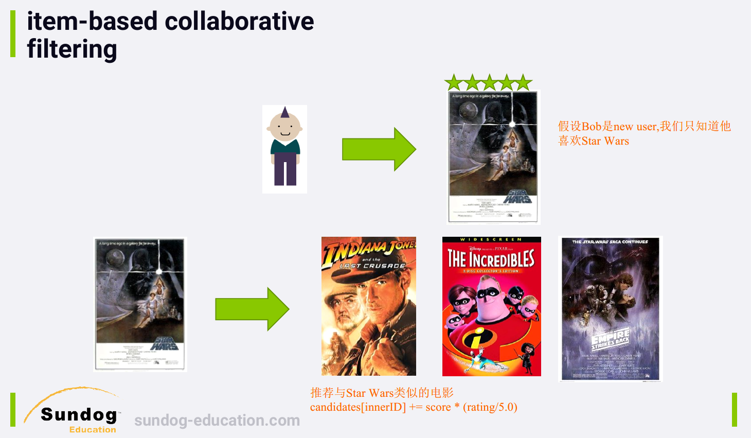
- 使用 item similarities also makes for a better experience for new users. 一个新用户只要表现出了对某个物品的兴趣,你可以推荐与那个物品相似的物品给该用户,而使用基于用户的协同过滤,you wouldn't have any recommendations for a new user at all until they make it into the next build of your user similarity matrix.
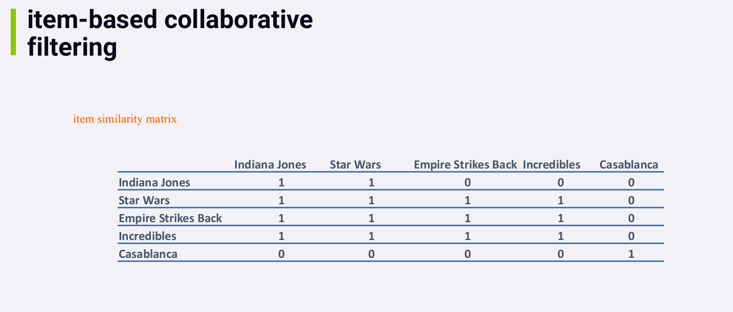
在这个例子中,所有的相似度都为0或1,是因为数据量比较小。In the real world, you'd see more interesting and meaningful numbers here.
3.2.1 计算物品相似度的方法
参考 https://github.com/NLP-LOVE/ML-NLP/tree/master/Project/17.%20Recommendation%20System
基于物品的协同过滤算法首先计算物品之间的相似度, 计算相似度的方法有以下几种:
1. 基于共同喜欢物品的用户列表计算
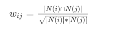
在此,分母中 \(N(i)\) 是购买物品 \(i\) 的用户数,\(N(j)\) 是购买物品 \(j\) 的用户数,而分子 \(N(i)∩N(j)\)是同时购买物品 \(i\) 和物品 \(j\) 的用户数。可见上述的公式的核心是计算同时购买这件商品的人数比例 。当同时购买这两个物品的人数越多,他们的相似度也就越高。另外值得注意的是,在分母中我们用了物品总购买人数做惩罚,也就是说某个物品可能很热门,导致它经常会被和其他物品一起购买,所以除以它的总购买人数,来降低它和其他物品的相似分数。
2. 基于余弦的相似度计算
上面的方法计算物品相似度是直接计算同时购买这两个物品的人数。但是也可能存在用户购买了但不喜欢的情况,所以如果数据集包含了具体的评分数据,我们可以进一步把用户评分引入到相似度计算中 。
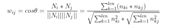
其中 \(n_{ki}\) 是用户 \(k\) 对物品 \(i\) 的评分,如果没有评分则为 0。
3. 热门物品的惩罚
对于热门物品的问题,可以用如下公式解决:
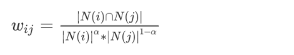
当 \(\alpha ∈ (0,0.5)\)时,\(N(i)\) 越小,惩罚得越厉害,从而会使热门物品相关性分数下降。
3.2.2 Item-based Collaborative Filtering, Hands-On
code walkthrough
CollaborativeFiltering文件夹里的:
运行SimpleItemCF.py
Item-based collaborative filtering is what Amazon used with outstanding success.
You need to test it out on several real people if possible, and then move to a large scale A/B test to see if this algorithm really is better or worse than whatever you might have today.
3.3 矩阵分解
参考 https://github.com/NLP-LOVE/ML-NLP/tree/master/Project/17.%20Recommendation%20System
上述计算会得到一个相似度矩阵,而这个矩阵的大小和维度都是很大的,需要进行降维处理,用到的是SVD的降维方法,具体可以参考:降维方法
基于稀疏自编码的矩阵分解
矩阵分解技术在推荐领域的应用比较成熟,但是通过上一节的介绍,我们不难发现矩阵分解本质上只通过一次分解来对原矩阵进行逼近,特征挖掘的层次不够深入。另外矩阵分解也没有运用到物品本身的内容特征,例如书本的类别分类、音乐的流派分类等。随着神经网络技术的兴起,笔者发现通过多层感知机,可以得到更加深度的特征表示,并且可以对内容分类特征加以应用。首先,我们介绍一下稀疏自编码神经网络的设计思路。
基础的自编码结构
最简单的自编码结构如下图,构造个三层的神经网络,我们让输出层等于输入层,且中间层的维度远低于输入层和输出层,这样就得到了第一层的特征压缩。
简单来说自编码神经网络尝试学习中间层约等于输入层的函数。换句话说,它尝试逼近一个恒等函数。如果网络的输入数据是完全随机的,比如每一个输入都是一个跟其他特征完全无关的独立同分布高斯随机变 ,那么这一压缩表示将会非常难于学习。但是如果输入数据中隐含着 些特定的结构,比如某些输入特征是彼此相关的,那么这一算法就可以发现输入数据中的这些相关性。
多层结构
基于以上的单层隐藏层的网络结构,我们可以扩展至多层网络结构,学习到更高层次的抽象特征。
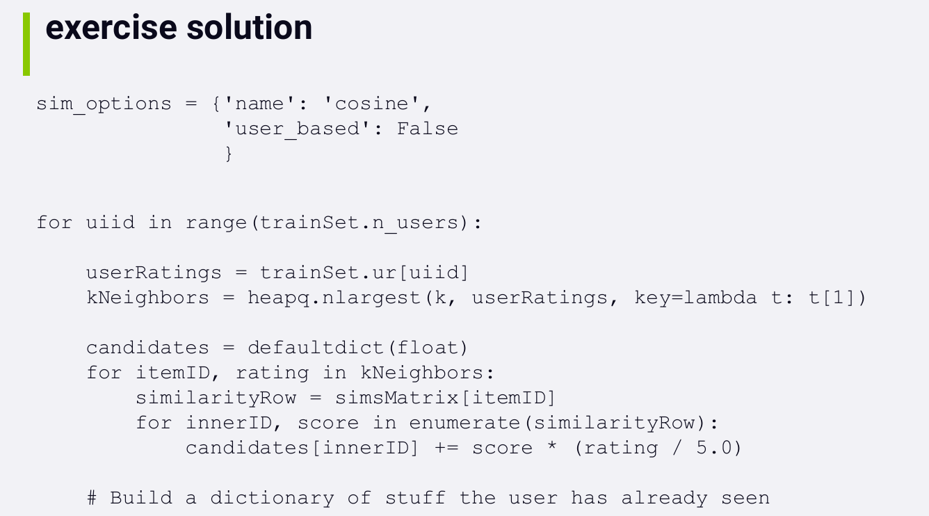
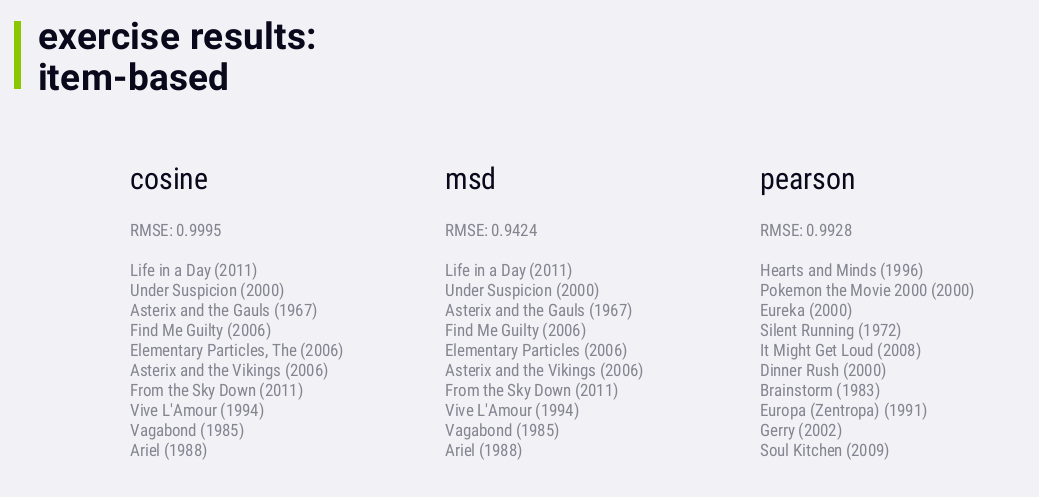
4. Exercise

我们之前是选取的top-n,例如item-based: 选择用户评价前10的电影,再找similar items;user-based: 选择与用户相似度排前10的用户,再...
Maybe it would be better if instead of taking the top k sources for recommendation candidates, we just use any source above some given quality threshold. 例如,用户评价4星以上的电影 should generate item-based recommendation candidates, no matter how many or how few of them there may be.
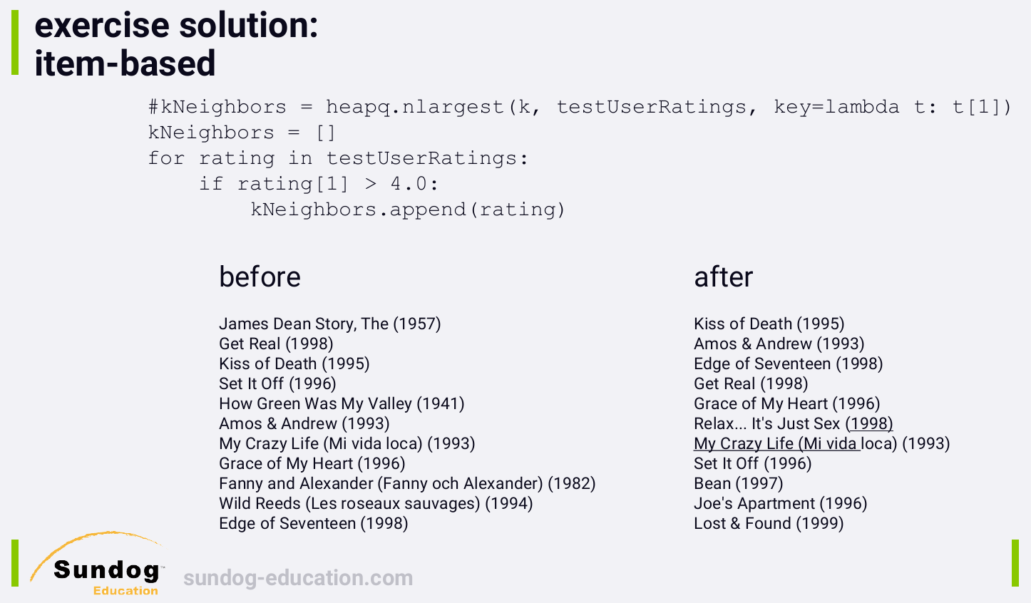
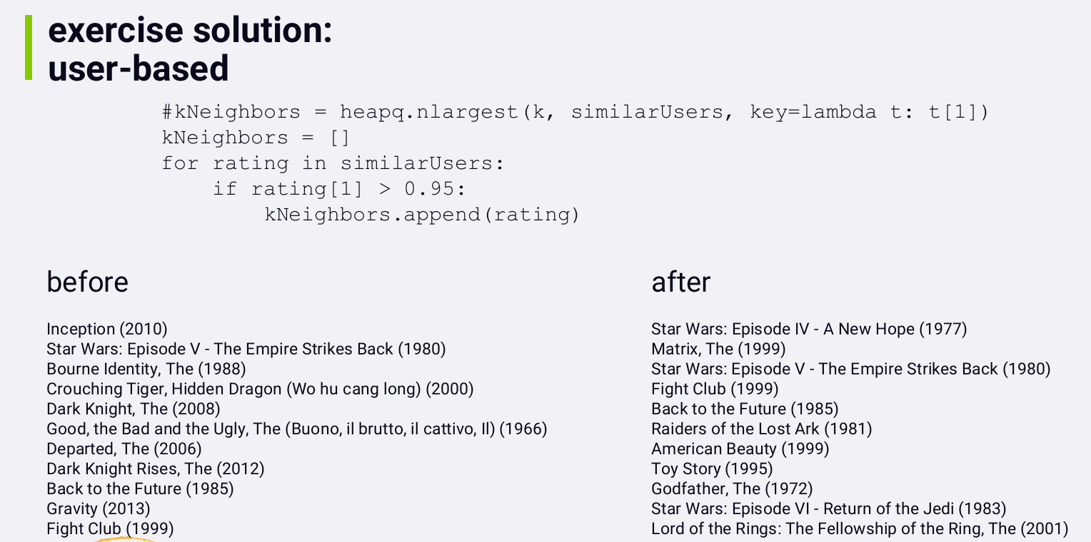
可以发现一个小的改变可以使得结果很不一样。Often, you don't just want to test different recommendation algorithms, you want to test different variations and parameters on those algorithms. In this case, I not only want to test the idea of using a threshold instead of a top k approach, I'd also want to test many different threshold values to find the best one. In the real world, you'll find that your biggest problem is just not having enough time to run all of the different experiments you want to run to make your recommendations better.
5. Evaluating Collaborative Filtering Systems Offline
Now, although we can't measure accuracy with user based or item based collaborative filtering, because they don't make rating predictions, we can still measure hit rate, because it is still a top-N recommender.
code walkthrough
CollaborativeFiltering文件夹里的:
运行EvaluateUserCF.py
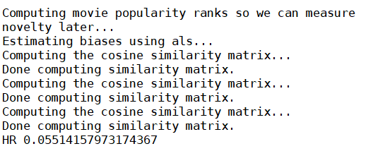
That was surprisingly fast. One really nice property of collaborative filtering is how quickly it can generate recommendations for any given individual, once we've built up the similarity matrix.
结果5.5% is pretty good.
Exercise
与EvaluateUserCF.py相比需要改变的地方:
item-based的hit rate只有0.5%,相比user-based的5.5%,要差一点。
Item-based should be a superior approach, and that's been proven in industry. 这里item-based要差一点应该是数据的原因。而且这只是offline evaluation. If we were to test both algorithms on real-world people using real-world data in an A/B test, the results could end up being very different.
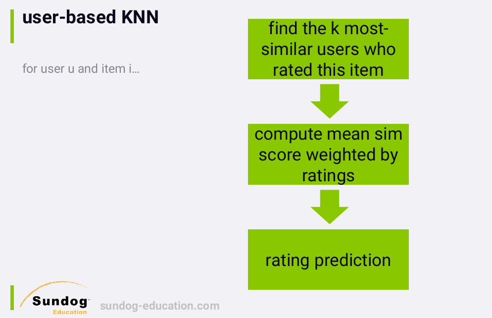
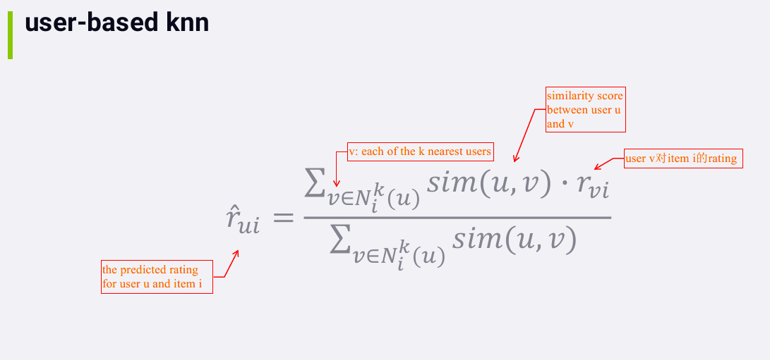
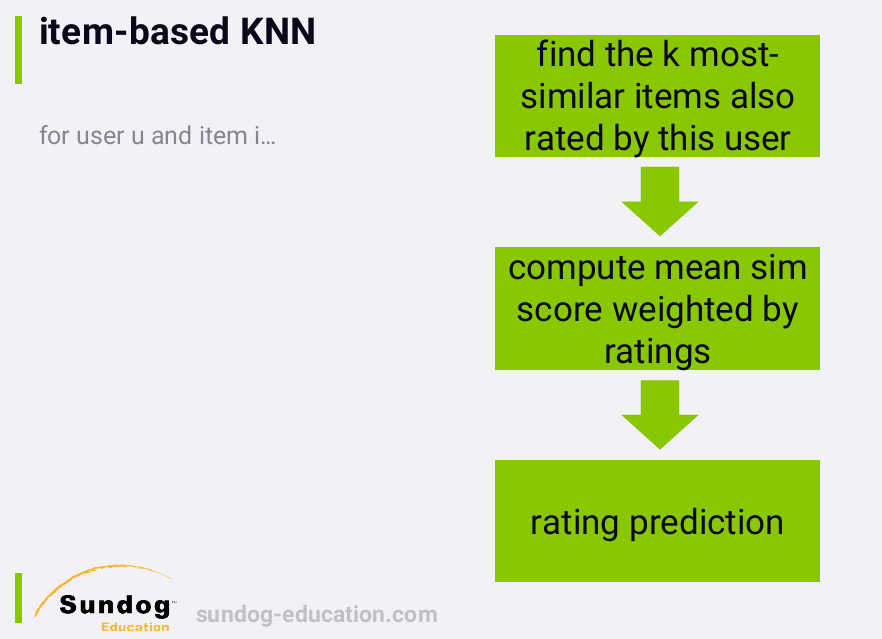
6. KNN Recommenders
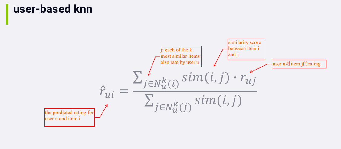
The concept of collaborative filtering has been applied to recommender systems that do make rating predictions, and these are generally referred to in the literature as KNN recommenders.
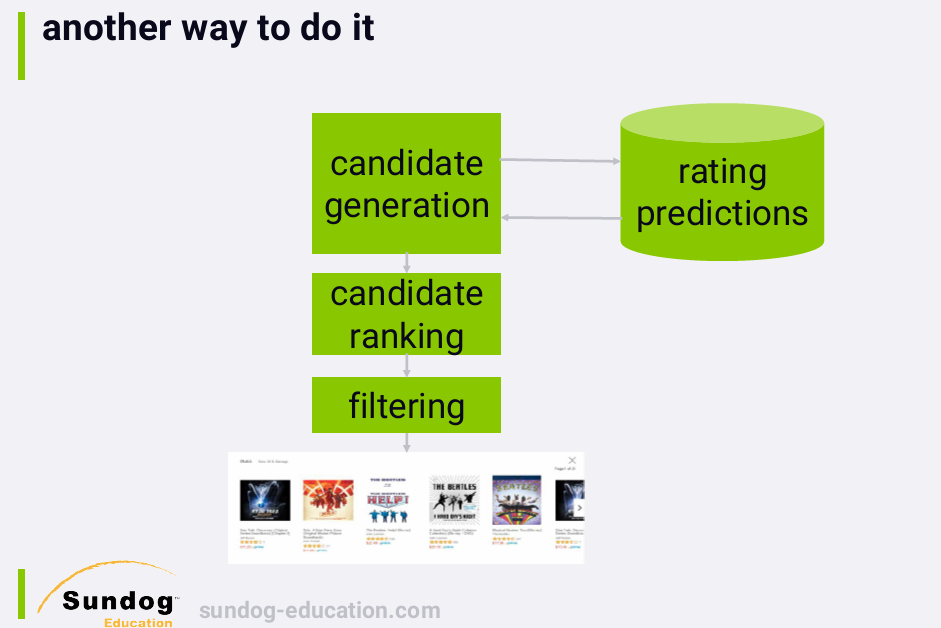
In this sort of system, we generate recommendation candidates by predicting the ratings of everything a user hasn't already rated, and selecting the top k items with the highest predicted ratings. This obviously isn't a terribly efficient approach, but since we're predicting rating values, we can measure the offline accuracy of the system using train/test or cross-validation, which is useful in the research world.
Running User and Item-based KNN on MovieLens
code walkthrough
CollaborativeFiltering文件夹里的:
运行KNNBakeOff.py
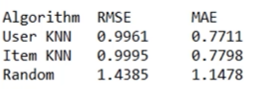
如果只看accuracy, KNN recommendation看上去是一个好方法,但是如果看 top-n recommendations, item-based和user-based推荐的都是些没听说过的电影 (obscure),反而 random recommendation looks a lot better from a subjective standpoint.
So, on the surface, it looks like we may have made a system that's pretty good at predicting ratings of movies people have already seen, but might not be very good at producing top-n recommendations.
Exercise
Experiment with different KNN parameters.

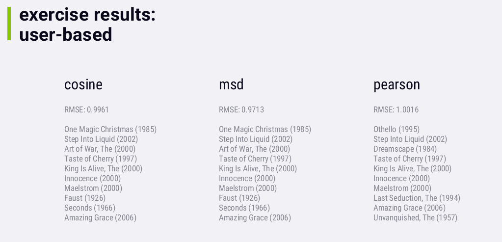
虽然msd比cosine的RMSE要低一点,但它们推荐的内容是一样的

Well, it's actually pretty well known that KNN doesn't work well in practice. Unfortunately, some people conclude that collaborative filtering in general is some naive approach that should be replaced with completely different techniques. But as we've seen, collaborative filtering isn't the problem, it's forcing collaborative filtering to make rating predictions -- that's the problem. We had some pretty exciting results when we just focused on making top-N recommendations, and completely forgot about optimizing for rating accuracy, and it turns out that's what at the heart of the problem. 使用user-based CF和item-based CF, top-N 推荐结果都是不错的。
Ratings are not continuous in nature, and KNN treats them as though they are continuous values that can be predicted on a continuous scale. If you really want to go with KNN, it would be more appropriate to treat it as a rating classification problem than as a rating prediction problem. KNN is also very sensitive to sparse data.
The most fundamental thing is that accuracy isn't everything. The main reason KNN produces underwhelming results is because it's trying to solve the wrong problem. KNN recommender之所以推荐结果不好,是因为它解决的是rating prediction的问题,而不是推荐问题。
7. Bleeding Edge Alert
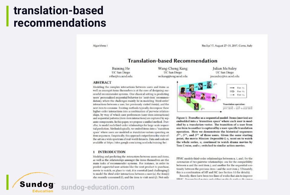

The idea behind it is that users are modeled as vectors moving from one item to another in a multidimensional space. And you can predict sequences of events, like which movie a user is likely to watch next, by modeling these vectors.
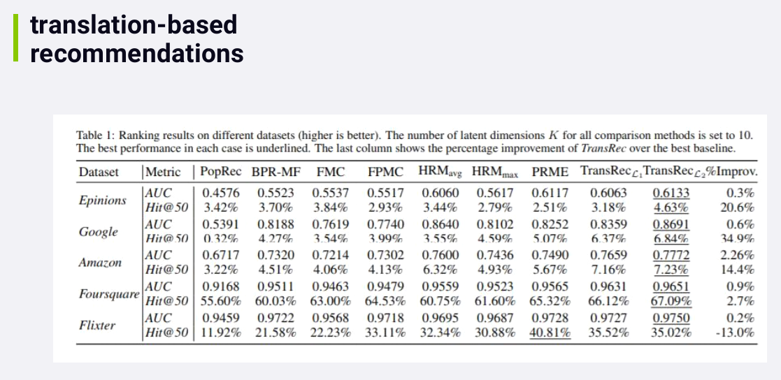
The reason this paper is exciting is because it outperformed all of the best existing methods for recommending sequences of events in all but one case in one data set.
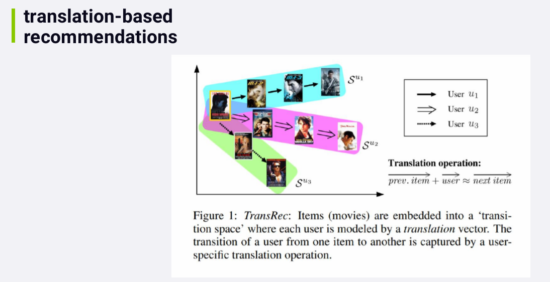
Basic idea: You position individual items, like movies, in a transition space, where neighborhoods within this space represent similarity between items. So items close together in this space are similar to each other. The dimensions corresponds to complex transition relationships between items. Since this technique depends on arranging items together into local, similar neighborhoods, I still classify it as a neighborhood -based method.
In this space, we can learn the vectors associated with individual users. Maybe a user who watches a Tom Cruise movie, is likely to move along to the next Tom Cruise movie, for example, and that transition would be represented by a vector in this space. We can then predict the next movie a user is like to watch by extrapolating along the vector we've associated with that user.
The paper provide the code in C++.
It's all very advanced stuff, but it seems to work. So if you find yourself in the situation where you need to predict a sequence of events, like which movies or videos a person is likely to watch next given theirs past history, you might wanna do a search for translation-based recommendations and how it's coming along in the real world.