Computer Vision
来源于Here’s your Learning Path to Master Computer Vision in 2020
1. Introduction
Face Recognition
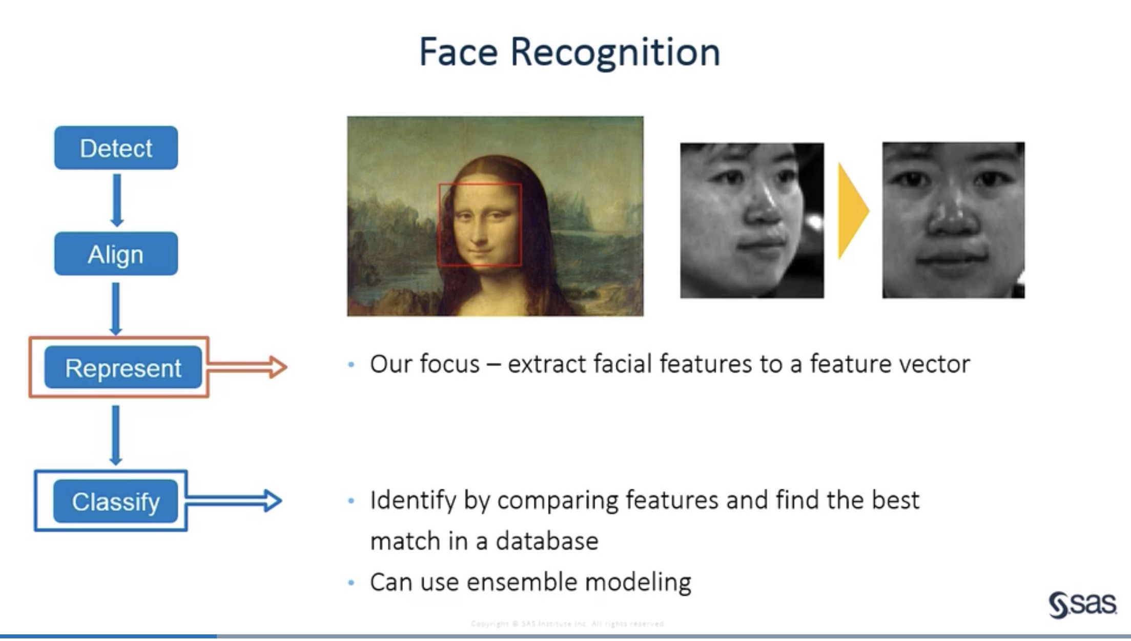
Types of computer vision
2. Image Preprocessing
2.1 Three Beginner-Friendly Techniques to Extract Features from Images
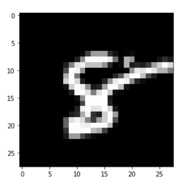
2.1.1 How do Machines Store Images?
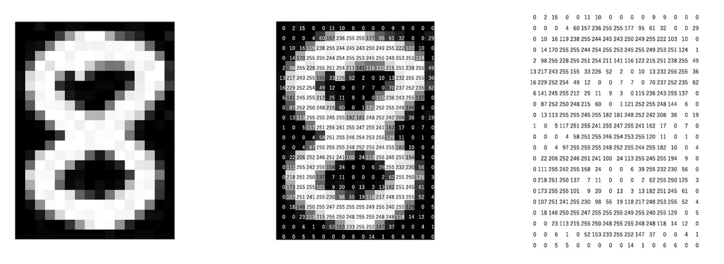
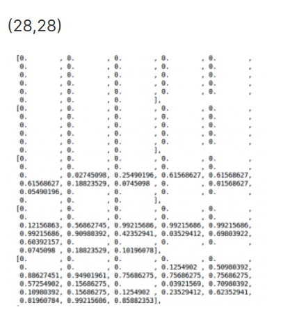
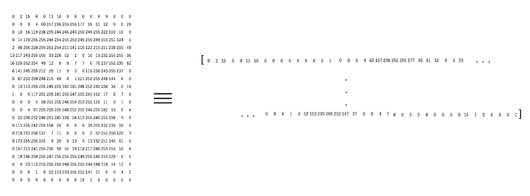
Machines store images in the form of a matrix of numbers. The size of this matrix depends on the number of pixels we have in any given image.
Let’s say the dimensions of an image are 180 x 200 or n x m. These dimensions are basically the number of pixels in the image (height x width).
These numbers, or the pixel values, denote the intensity or brightness of the pixel. Smaller numbers (closer to 0) represent black, and larger numbers (closer to 255) denote white. You’ll understand whatever we have learned so far by analyzing the below image.
The dimensions of the below image are 22 x 16, which you can verify by counting the number of pixels:
以上讨论的是黑白图片,那么彩色图片呢? 彩色图片依旧以二维矩阵的形式存储吗?
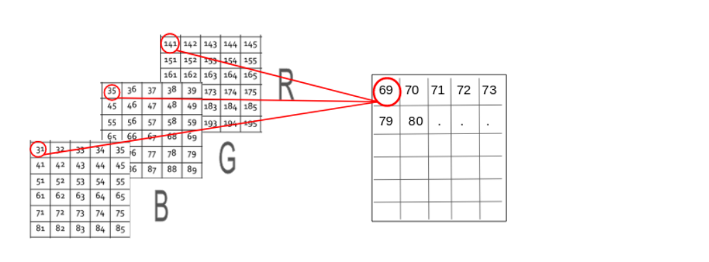
A colored image is typically composed of multiple colors and almost all colors can be generated from three primary colors – red, green and blue.
In the case of a colored image, there are three Matrices (or channels) – Red, Green, and Blue. Each matrix has values between 0-255 representing the intensity of the color for that pixel. Consider the below image to understand this concept:
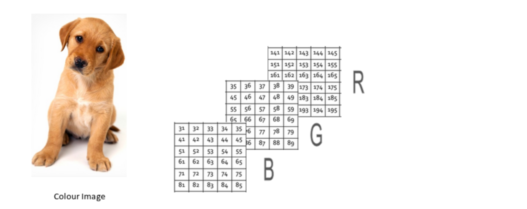
The three channels are superimposed (叠加) to form a colored image.
Note that these are not the original pixel values for the given image as the original matrix would be very large and difficult to visualize. Also, there are various other formats in which the images are stored. RGB is the most popular one and hence I have addressed it here. You can read more about the other popular formats here.
2.1.2 Reading Image Data in Python
1 | import pandas as pd |
1 | #checking image shape |
Let’s now explore various methods of using pixel values as features.
2.1.3 Method #1: Grayscale Pixel Values as Features
The simplest way to create features from an image is to use these raw pixel values as separate features.
特征的维度等于pixels的数量
How do we arrange these pixels as features? Well, we can simply append every pixel value one after the other to generate a feature vector. 如下图所示:
Let us take an image in Python and create these features for that image:
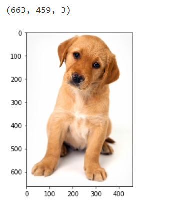
1 | image = imread('puppy.jpeg', as_gray=True) |
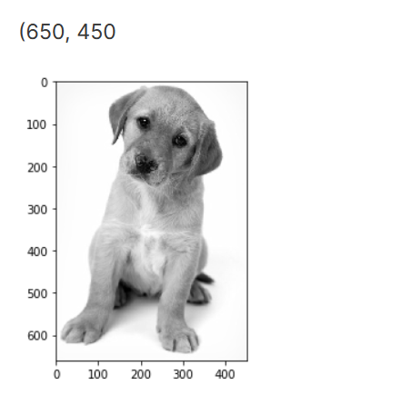
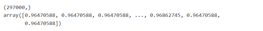
The image shape here is 660 x 450. Hence, the number of features
should be 297,000. We can generate this using the reshape
function from NumPy where we specify the dimension of the image:
1 | #pixel features |
But here, we only had a single channel or a grayscale image. Can we do the same for a colored image? Let’s find out!
2.1.4 Method #2: Mean Pixel Value of Channels (Colored Image)
While reading the image in the previous section, we had set the
parameter as_gray = True. So we only had one channel in the
image and we could easily append the pixel values. Let us remove the
parameter and load the image again:
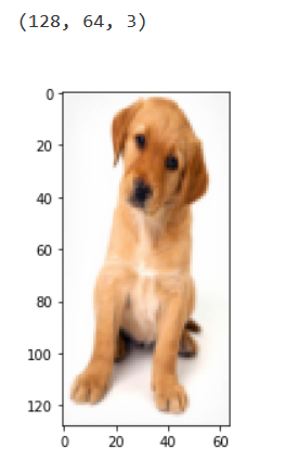
1 | image = imread('puppy.jpeg') |
1 | (660, 450, 3) |
This time, the image has a dimension (660, 450, 3), where 3 is the number of channels. We can go ahead and create the features as we did previously. The number of features, in this case, will be 660*450*3 = 891,000.
Alternatively, here is another approach we can use:
Instead of using the pixel values from the three channels separately, we can generate a new matrix that has the mean value of pixels from all three channels.
如下图所示:(取均值)
By doing so, the number of features remains the same and we also take into account the pixel values from all three channels of the image.
1 | image = imread('puppy.jpeg') |
The new matrix will have the same height and width but only 1 channel. Now we can follow the same steps that we did in the previous section. We append the pixel values one after the other to get a 1D array:
1 | features = np.reshape(feature_matrix, (660*450)) |
1 | (297000,) |
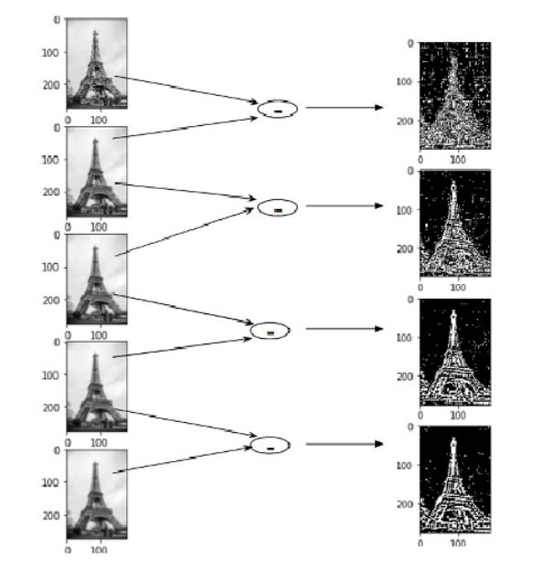
2.1.5 Method #3: Extracting Edge Features
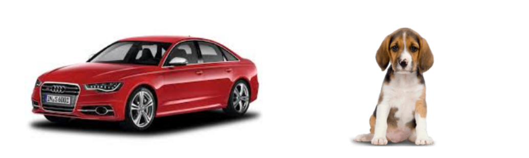
假设我们有下面的图像,我们需要识别其中的物体:
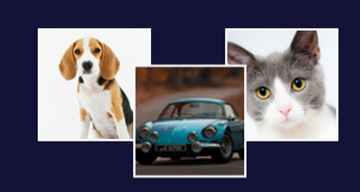
你一定在一瞬间就认出了这些物体——狗、车和猫。在区分这些图像时,你考虑了哪些特征?The shape could be one important factor, followed by color, or size. What if the machine could also identify the shape as we do?
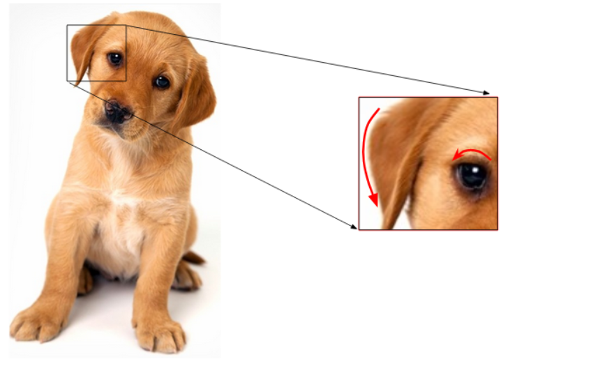
A similar idea is to extract edges as features and use that as the input for the model. I want you to think about this for a moment – 如何识别图片中的edges? Edge is basically where there is a sharp change in color. Look at the below image:
And as we know, an image is represented in the form of numbers. So, we will look for pixels around which there is a drastic change in the pixel values. (像素点周围的数值是否有很大的变化)
Let’s say we have the following matrix for the image:
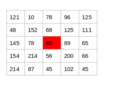
To identify if a pixel is an edge or not, we will simply subtract the values on either side of the pixel. For this example, we have the highlighted value of 85. We will find the difference between the values 89 and 78. Since this difference is not very large, we can say that there is no edge around this pixel.
Now consider the pixel 125 highlighted in the below image:
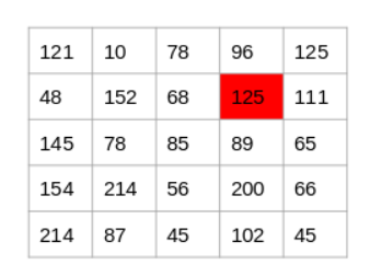
Since the difference between the values on either side of this pixel is large, we can conclude that there is a significant transition at this pixel and hence it is an edge. Now the question is, do we have to do this step manually?
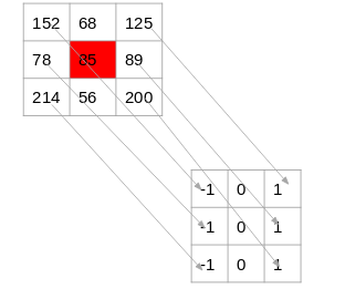
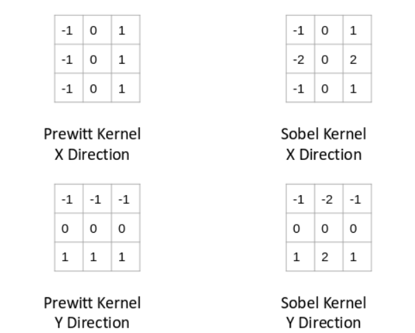
No! There are various kernels that can be used to highlight the edges in an image. The method we just discussed can also be achieved using the Prewitt kernel (in the x-direction). Given below is the Prewitt kernel:
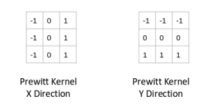
We take the values surrounding the selected pixel and multiply it with the selected kernel (Prewitt kernel). We can then add the resulting values to get a final value. Since we already have -1 in one column and 1 in the other column, adding the values is equivalent to taking the difference.
There are various other kernels and I have mentioned four most popularly used ones below:
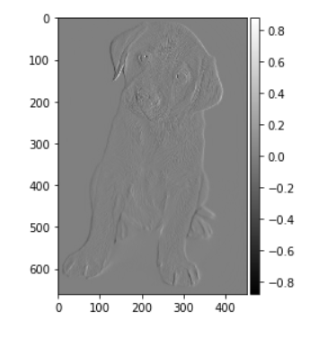
Let’s now go back to the notebook and generate edge features for the same image:
1 | #importing the required libraries |
2.1.6 Key Takeawys
- 图像存储为像素值矩阵,彩色图像具有单独的通道(R, G, B)
- 简单的特征提取技术包括使用原始像素值、跨通道的平均像素值和边缘检测
- 图像的特征提取是将机器学习模型应用于图像数据和计算机视觉任务的关键步骤
2.2 HOG (Histogram of Oriented Gradients) features
2.2.1 What is a Feature Descriptor?
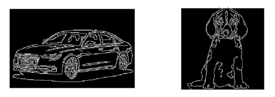
第一组图像有很多信息,比如物体的形状、颜色、边缘、背景等,第二组图像的信息要少得多(只有形状和边缘),但仍然足以区分这两幅图像。
We were easily able to differentiate the objects in the second case because it had the necessary information we would need to identify the object. And that is exactly what a feature descriptor does:
它是图像的简化表示,仅包含有关图像的最重要的信息
There are a number of feature descriptors out there. Here are a few of the most popular ones:
- HOG: Histogram of Oriented Gradients
- SIFT: Scale Invariant Feature Transform
- SURF: Speeded-Up Robust Feature
2.2.2 Introduction to the HOG Feature Descriptor
HOG, or Histogram of Oriented Gradients, is a feature descriptor that is often used to extract features from image data. It is widely used in computer vision tasks for object detection.
让我们看一看使得HOG与其他 feature descriptor 不同的一些重要方面:
- The HOG descriptor focuses on the structure or the shape of an object. Now you might ask, how is this different from the edge features we extract for images? In the case of edge features, we only identify if the pixel is an edge or not. HOG is able to provide the edge direction as well. This is done by extracting the gradient and orientation (or you can say magnitude and direction) of the edges
- Additionally, these orientations are calculated in ‘localized’ portions. This means that the complete image is broken down into smaller regions and for each region, the gradients and orientation are calculated. We will discuss this in much more detail in the upcoming sections
- Finally the HOG would generate a Histogram for each of these regions separately. The histograms are created using the gradients and orientations of the pixel values, hence the name ‘Histogram of Oriented Gradients’
HOG的正式定义:
The HOG feature descriptor counts the occurrences of gradient orientation in localized portions of an image.
Implementing HOG using tools like OpenCV is extremely simple. It’s just a few lines of code since we have a predefined function called hog in the skimage.feature library. Our focus in this article, however, is on how these features are actually calculated.
2.2.3 Process of Calculating the Histogram of Oriented Gradients (HOG)
HOG具体是怎么计算的:详细内容见这里.
2.2.4 Implementing HOG Feature Descriptor in Python
1 | #importing required libraries |
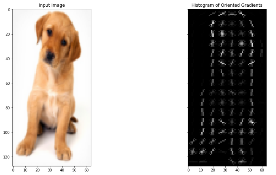
We can see that the shape of the image is 663 x 459. We will have to
resize this image into 64 x 128. Note that we are using
skimage which takes the input as height x width.
1 | #resizing image |
Here, I am going to use the hog function from
skimage.feature directly. So we don’t have to calculate the
gradients, magnitude (total gradient) and orientation individually. The
hog function would internally calculate it and return the feature
matrix.
Also, if you set the parameter visualize = True, it will
return an image of the HOG.
1 | #creating hog features |
Before going ahead, let me give you a basic idea of what each of these hyperparameters represents. Alternatively, you can check the definitions from the official documentation here.
- The
orientationsare the number of buckets we want to create. Since I want to have a 9 x 1 matrix, I will set the orientations to 9 pixels_per_celldefines the size of the cell for which we create the histograms. In the example we covered in this article, we used 8 x 8 cells and here I will set the same value. As mentioned previously, you can choose to change this value- We have another hyperparameter
cells_per_blockwhich is the size of the block over which we normalize the histogram. Here, we mention the cells per blocks and not the number of pixels. So, instead of writing 16 x 16, we will use 2 x 2 here
The feature matrix from the function is stored in the variable
fd, and the image is stored in hog_image. Let
us check the shape of the feature matrix:
1 | fd.shape |
(3780,)
As expected, we have 3,780 features for the image and this verifies the calculations we did in step 7 earlier. You can choose to change the values of the hyperparameters and that will give you a feature matrix of different sizes.
Let’s finally look at the HOG image:
1 | fig, (ax1, ax2) = plt.subplots(1, 2, figsize=(16, 8), sharex=True, sharey=True) |
2.2.5 Conclusion
这一节的主要内容是介绍了 HOG feature descriptor 背后实际发生了什么,以及特征是如何计算的。 As a next step, we would encourage you to try using HOG features on a simple computer vision problem and see if the model performance improves.
2.3 SIFT (Scale Invariant Feature Transform) features
看看下面的图片集合,它们之间的共同元素是什么:
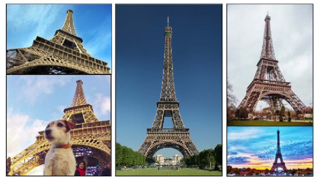
当然是金碧辉煌的埃菲尔铁塔!我们自然会明白,图像的比例或角度可能会改变,但物体是不变的。
But machines have an almighty struggle with the same idea. It’s a challenge for them to identify the object in an image if we change certain things (like the angle or the scale). Here’s the good news – machines are super flexible and we can teach them to identify images at an almost human-level.
So, in this article, we will talk about an image matching algorithm that identifies the key features from the images and is able to match these features to a new image of the same object.
2.3.1 Introduction to SIFT
SIFT, or Scale Invariant Feature Transform, is a feature detection algorithm in Computer Vision.
SIFT helps locate the local features in an image, commonly known as the ‘keypoints‘ of the image. These keypoints are scale & rotation invariant that can be used for various computer vision applications, like image matching, object detection, scene detection, etc.
在模型训练过程中,我们也可以使用SIFT生成的关键点作为图像的特征。SIFT features (over edge features or hog features)的主要优点是它们不受图像大小或方向的影响。
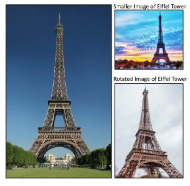
For example, here is another image of the Eiffel Tower along with its smaller version. The keypoints of the object in the first image are matched with the keypoints found in the second image. The same goes for two images when the object in the other image is slightly rotated. Amazing, right?
接下来让我们了解如何识别这些关键点,以及用于确保缩放和旋转不变性的技术是什么。总的来说,整个过程可以分为4个部分:
- Constructing a Scale Space: To make sure that features are scale-independent
- Keypoint Localisation (关键点定位): Identifying the suitable features or keypoints
- Orientation Assignment: Ensure the keypoints are rotation invariant
- Keypoint Descriptor: Assign a unique fingerprint to each keypoint
Finally, we can use these keypoints for feature matching!
This article is based on the original paper by David G. Lowe. Here is the link: Distinctive Image Features from Scale-Invariant Keypoints.
2.3.2 Constructing the Scale Space
我们需要识别给定图像中最明显的特征,同时忽略任何噪声。此外,我们需要确保这些特征 are not scale-dependent.
1.reduce the noise
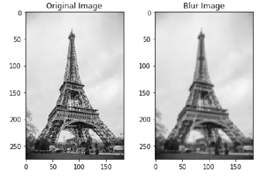
We use the Gaussian Blurring technique to reduce the noise in an image.
So, for every pixel in an image, the Gaussian Blur calculates a value based on its neighboring pixels. Below is an example of image before and after applying the Gaussian Blur. As you can see, the texture and minor details are removed from the image and only the relevant information like the shape and edges remain:
2.ensure the features are not scale-dependent
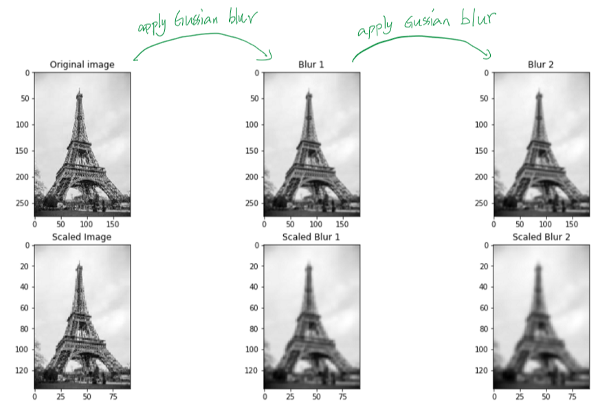
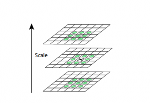
Gaussian Blur successfully removed the noise from the images and we have highlighted the important features of the image. Now, we need to ensure that these features must not be scale-dependent. This means we will be searching for these features on multiple scales, by creating a ‘scale space’.
Scale space is a collection of images having different scales, generated from a single image.
To create a new set of images of different scales, we will take the original image and reduce the scale by half. For each new image, we will create blur versions as we saw above.
例:We have the original image of size (275, 183) and a scaled image of dimension (138, 92). For both the images, two blur images are created:
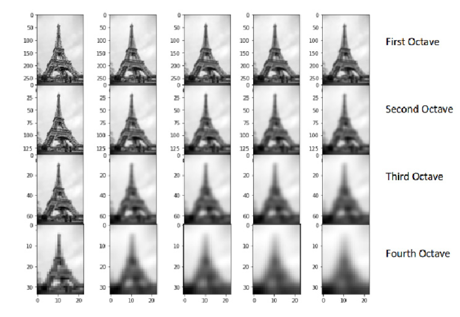
How many times do we need to scale the image and how many subsequent blur images need to be created for each scaled image? The ideal number of octaves should be four, and for each octave, the number of blur images should be five.
Difference of Gaussian
So far we have created images of multiple scales (often represented by σ) and used Gaussian blur for each of them to reduce the noise in the image. Next, we will try to enhance the features using a technique called Difference of Gaussians or DoG.
Difference of Gaussian is a feature enhancement algorithm that involves the subtraction of one blurred version of an original image from another, less blurred version of the original.
DoG creates another set of images, for each octave, by subtracting every image from the previous image in the same scale.
Let us create the DoG for the images in scale space. 如下图所示,On the left, we have 5 images, all from the first octave (thus having the same scale). Each subsequent image is created by applying the Gaussian blur over the previous image. On the right, we have four images generated by subtracting the consecutive Gaussians. The results are jaw-dropping (让人吃惊)!
Now that we have a new set of images, we are going to use this to find the important keypoints.
2.3.3 Keypoint Localization (关键点定位)
一旦创建了图像,下一步就是从图像中找到可用于特征匹配的重要关键点 (keypoints)。 The idea is to find the local maxima and minima for the images. This part is divided into two steps:
Local Maxima and Local Minima
To locate the local maxima and minima, we go through every pixel in the image and compare it with its neighboring pixels.
When I say ‘neighboring’, this not only includes the surrounding pixels of that image (in which the pixel lies), but also the nine pixels for the previous and next image in the octave.
This means that every pixel value is compared with 26 other pixel values to find whether it is the local maxima/minima. For example, in the below diagram, we have three images from the first octave. The pixel marked x is compared with the neighboring pixels (in green) and is selected as a keypoint if it is the highest or lowest among the neighbors:
We now have potential keypoints that represent the images and are scale-invariant. 我们将在选定的关键点上应用最后一次检查(keypoint selection),以确保这些是用来表示图像的最准确的关键点。(因为其中一些关键点可能对噪声不太robust。)
Keypoint Selection
我们将消除低对比度的关键点,或者非常靠近边缘的关键点。
To deal with the low contrast keypoints, a second-order Taylor expansion is computed for each keypoint. If the resulting value is less than 0.03 (in magnitude), we reject the keypoint.
对于剩下的关键点,我们会进行检查,找出位置不佳的关键点。这些是接近边缘的关键点,具有高边缘响应,但可能对少量噪声不够稳健。用二阶Hessian矩阵来识别这些关键点。
Now that we have performed both the contrast test and the edge test to reject the unstable keypoints, we will now assign an orientation value for each keypoint to make the rotation invariant.
2.3.4 Orientation Assignment
At this stage, we have a set of stable keypoints for the images. We will now assign an orientation to each of these keypoints so that they are invariant to rotation. We can again divide this step into two smaller steps:
- Calculate the magnitude and orientation
- Create a histogram for magnitude and orientation
计算magnitude和orientation的方法与 HOG中的计算方法类似,具体计算过程见这里.
The magnitude represents the intensity of the pixel and the orientation gives the direction for the same.
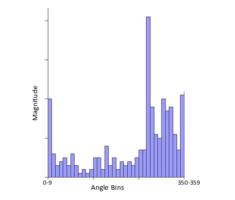
Creating a Histogram for Magnitude and Orientation
On the x-axis, we will have bins for angle values, like 0-9, 10 – 19, 20-29, up to 360. Since our angle value is 57, it will fall in the 6th bin. The 6th bin value will be in proportion to the magnitude of the pixel, i.e. 16.64. We will do this for all the pixels around the keypoint.
This is how we get the below histogram:
You can refer to this article for a much detailed explanation for calculating the gradient, magnitude, orientation and plotting histogram – A Valuable Introduction to the Histogram of Oriented Gradients.
This histogram would peak at some point. The bin at which we see the peak will be the orientation for the keypoint. Additionally, if there is another significant peak (seen between 80 – 100%), then another keypoint is generated with the magnitude and scale the same as the keypoint used to generate the histogram. And the angle or orientation will be equal to the new bin that has the peak.
Effectively at this point, we can say that there can be a small increase in the number of keypoints.
2.3.5 Keypoint Descriptor
This is the final step for SIFT. So far, we have stable keypoints that are scale-invariant and rotation invariant. In this section, we will use the neighboring pixels, their orientations, and magnitude, to generate a unique fingerprint for this keypoint called a ‘descriptor’.
Additionally, since we use the surrounding pixels, the descriptors will be partially invariant to illumination or brightness of the images.
We will first take a 16×16 neighborhood around the keypoint. This 16×16 block is further divided into 4×4 sub-blocks and for each of these sub-blocks, we generate the histogram using magnitude and orientation.
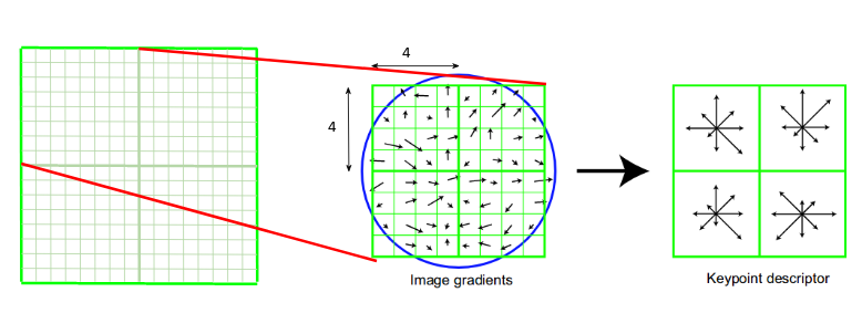
At this stage, the bin size is increased and we take only 8 bins (not 36). Each of these arrows represents the 8 bins and the length of the arrows define the magnitude. So, we will have a total of 128 bin values for every keypoint.
Here is an example:
1 | import cv2 |
2.3.6 Feature Matching (代码)
We will now use the SIFT features for feature matching. For this
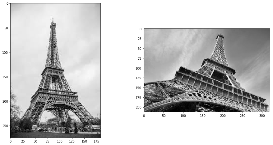
purpose, I have downloaded two images of the Eiffel Tower, taken from
different positions. You can try it with any two images that you want.
Here are the two images that I have used:
1 | import cv2 |
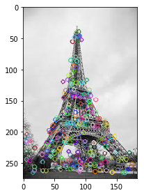
Now, for both these images, we are going to generate the SIFT features. First, we have to construct a SIFT object and then use the function detectAndCompute to get the keypoints. It will return two values – the keypoints and the descriptors.
Let’s determine the keypoints and print the total number of keypoints found in each image:
1 | import cv2 |
283, 540
Next, let’s try and match the features from image 1 with features
from image 2. We will be using the function match() from
the BFmatcher (brute force match) module. Also, we will draw
lines between the features that match in both the images. This can be
done using the drawMatches() function in OpenCV.
1 | import cv2 |
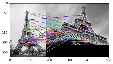
I have plotted only 50 matches here for clarity’s sake. You can
increase the number according to what you prefer. To find out how many
keypoints are matched, we can print the length of the variable
matches. In this case, the answer would be 190.
2.3.7 End Notes
In this article, we discussed the SIFT feature matching algorithm in detail. Here is a site that provides excellent visualization for each step of SIFT. You can add your own image and it will create the keypoints for that image as well. Check it out here.
Another popular feature matching algorithm is SURF (Speeded Up Robust Feature), which is simply a faster version of SIFT. I would encourage you to go ahead and explore it as well.
And if you’re new to the world of computer vision and image data, I recommend checking out the below course:
3. Image Classification using Logistic Regression
Python:
kaggle kernel: used grid search method in logistic regression to classify rooms as messy or clean.
完整代码见:https://www.kaggle.com/gulsahdemiryurek/image-classification-with-logistic-regression/notebook
对图片的大致处理:(在这里,先不纠结train/val/test等)
1 | import numpy as np |
1 | def train_data(): |
1 | train_data = train_data() |
1 | x_train_flatten = train_data.reshape(train_data.shape[0],train_data.shape[1]*train_data.shape[2]) |
Grid search:
1 | from sklearn.linear_model import LogisticRegression |
- C: Using Logistic regression to classify images (MNIST data)
4. Project 1- Identify the Apparels (服装)

More than 25% of entire revenue in E-Commerce is attributed to apparels & accessories. A major problem they face is categorizing these apparels from just the images especially when the categories provided by the brands are inconsistent. This poses an interesting computer vision problem which has caught the eyes of several deep learning researchers.
Fashion MNIST is a drop-in replacement for the very well known, machine learning hello world - MNIST dataset which can be checked out at ‘Identify the digits’ practice problem. Instead of digits, the images show a type of apparel e.g. T-shirt, trousers, bag, etc. The dataset used in this problem was created by Zalando Research. More details can be found at this link.
5. Introduction to Keras & Neural Networks
5.1 Keras
Keras is one of the most commonly used deep learning tools.
- Keras Documentation (Keras官方文档)
- Neural Networks using Keras (MNIST)
5.2 Neural Network
Introduction to Neural Networks by Stanford:
Neural Networks by 3Blue1Brown:
6. Project 1 - Identify the Apparels
同第4部分
7. Understanding CNNs, Transfer Learning
7.1 Introduction to Convolutional Neural Networks (CNNs):
Convolutional Neural Networks by Stanford:
7.2 Introduction to Transfer Learning:
7.2.1 Master Transfer Learning
训练神经网络有时需要很多的资源(RAM, GPUs), RAM on a machine is cheap and is available in plenty, but access to GPUs is not that cheap.
这种情况在未来可能会改变。但就目前而言,这意味着我们必须更明智地使用我们的资源来解决深度学习问题。尤其是当我们试图解决复杂的现实生活问题时,比如图像和语音识别。Once you have a few hidden layers in your model, adding another layer of hidden layer would need immense resources.
Thankfully, there is something called “Transfer Learning” which enables us to use pre-trained models from other people by making small changes. In this article, I am going to tell how we can use pre-trained models to accelerate our solutions.
- What is transfer learning?
A neural network is trained on a data. This network gains knowledge from this data, which is compiled as “weights” of the network. These weights can be extracted and then transferred to any other neural network. Instead of training the other neural network from scratch, we “transfer” the learned features.
- What is a Pre-trained Model?
简单地说,预训练模型是由其他人为解决类似问题而创建的模型。对于我们来说,可以不再从头开始构建模型来解决类似的问题,而是可以使用在其他问题上训练过的模型作为起点。
比如,如果你想造一辆
self learning
car。你可以花几年的时间从头开始构建一个像样的图像识别算法,或者 you can
take inception model (a pre-trained model) from Google which was built
on ImageNet data to identify images in those pictures.
A pre-trained
model may not be 100% accurate in your application, but it saves huge
efforts required to re-invent the wheel.
使用pre-trained model不仅能节约训练时间,还能得到更高的准确率
- How can I use Pre-trained Models?
通过使用预先在大型数据集上训练过的预训练模型,我们可以直接使用获得的权重和 architecture, and apply the learning on our problem statement. This is known as transfer learning. We “transfer the learning” of the pre-trained model to our specific problem statement.
在选择在您的案例中应该使用的预训练模型时,您应该非常小心。如果我们手头的问题陈述与预训练模型所训练的问题陈述非常不同,那么我们得到的预测将非常不准确。For example, a model previously trained for speech recognition would work horribly if we try to use it to identify objects using it.
We are lucky that many pre-trained architectures are directly available for us in the Keras library. Imagenet data set has been widely used to build various architectures since it is large enough (1.2M images) to create a generalized model. The problem statement is to train a model that can correctly classify the images into 1,000 separate object categories. These 1,000 image categories represent object classes that we come across in our day-to-day lives, such as species of dogs, cats, various household objects, vehicle types etc.
These pre-trained networks demonstrate a strong ability to generalize to images outside the ImageNet dataset via transfer learning. We make modifications in the pre-existing model by fine-tuning the model. Since we assume that the pre-trained network has been trained quite well, we would not want to modify the weights too soon and too much. While modifying we generally use a learning rate smaller than the one used for initially training the model.
Ways to Fine tune the model
- Feature extraction – We can use a pre-trained model as a feature extraction mechanism. What we can do is that we can remove the output layer( the one which gives the probabilities for being in each of the 1000 classes) and then use the entire network as a fixed feature extractor for the new data set.
- Use the Architecture of the pre-trained model – We use architecture of the model while we initialize all the weights randomly and train the model according to our dataset again.
- Train some layers while freeze others – Another way to use a pre-trained model is to train it partially. We keep the weights of initial layers of the model frozen while we retrain only the higher layers. We can try and test as to how many layers to be frozen and how many to be trained.
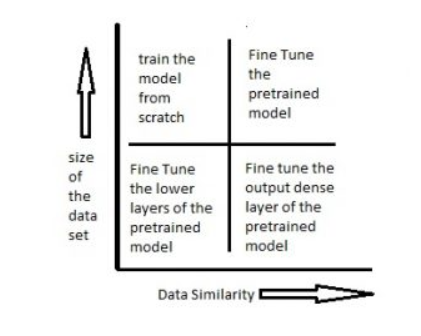
Scenario 1 – Size of the Data set is small while the Data similarity is very high (右下角) – 在这种情况下,由于数据相似度非常高,我们不需要重新训练模型。我们所需要做的就是根据问题陈述 customize and modify 输出层。We use the pretrained model as a feature extractor. 假设我们决定使用在Imagenet上训练的模型来识别 new set of images 是猫还是狗。(需要识别的图像类似于Imagenet,但是只需要两个类别作为输出 —— 猫或狗。)In this case all we do is just modify the dense layers and the final softmax layer to output 2 categories instead of a 1000.
Scenario 2 – Size of the data is small as well as data similarity is very low (左下角) – 在这种情况下,我们可以冻结预训练模型的初始(假设k)层,并再次训练剩余的(n-k)层。The top layers would then be customized to the new data set. 由于新数据集具有较低的相似度,因此根据新数据集重新训练和自定义更高层具有重要意义。数据集较小通过以下事实得到补偿 (compensate) :初始层保持预训练(之前已经在大型数据集上训练过),并且这些层的权重被冻结。
Scenario 3 – Size of the data set is large however the Data similarity is very low (左上角) – 在这种情况下,由于我们数据集较大,我们的神经网络训练将是有效的。然而,由于我们拥有的数据与用于训练预训练模型的数据非常不同,使用预训练模型做出的预测 would not be effective。因此,最好根据你的数据从头开始训练神经网络。
Scenario 4 – Size of the data is large as well as there is high data similarity (右上角) – This is the ideal situation. In this case the pretrained model should be most effective. The best way to use the model is to retain the architecture of the model and the initial weights of the model. Then we can retrain this model using the weights as initialized in the pre-trained model.
There are various architectures that have been trained on the imageNet data set. You can go through various architectures here.
代码示例: use the pre-trained models to identify handwritten digits. 见这里
7.2.2 ConvNets in Practice by Stanford
8. Project 2 - Idendify the Digits
Automatic digit recognition is of popular interest today. Deep Learning techniques makes it possible for object recognition in image data. This practice problem is meant to give you a kick start in deep learning. As usual, we will not only provide you with the challenge and a solution checker, but also a set of tutorials to get you off the ground!
The data set used for this problem is from the populat MNIST data set. Developed by Yann LeCun, Corina Cortes and Christopher Burger for evaluating machine learning model on the handwritten digit classification problem. It is a widely used data set in the machine learning community. For more details about the data set, read here http://bit.ly/1REjJgL
9. Build your profile: Participate in competitions
10. Solving Object Detection problems
10.1 Step-by-Step Introduction to Object Detection Techniques
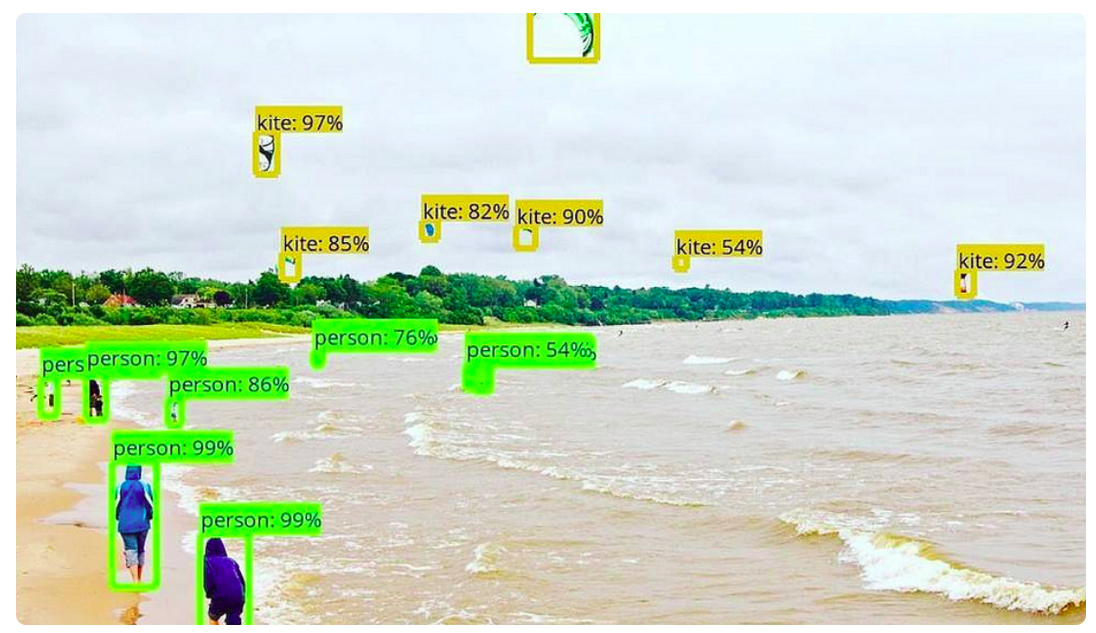
下图是一个很流行的例子,说明了目标检测算法是如何工作的。图像中的每个物体,从人到风筝,都以一定的精度被定位和识别。
让我们看看如何使用CNN来解决一般的目标检测问题。
首先,我们将图像作为输入
然后将图像划分为不同的区域
然后,我们将把每个区域视为一个单独的图像。
将所有这些 regions (images) 传递给CNN,并将其分类为不同的类。
一旦我们将每个区域划分为相应的类,我们就可以将所有这些区域组合起来,得到带有检测对象的原始图像
使用这种方法的问题是,图像中的物体可能具有不同的长宽比和空间位置。例如,在某些情况下,物体可能覆盖了图像的大部分,而在其他情况下,物体可能只覆盖了图像的一小部分。物体的形状也可能不同(在实际用例中经常发生)。
As a result of these factors, we would require a very large number of regions resulting in a huge amount of computational time. So to solve this problem and reduce the number of regions, we can use region-based CNN (RCNN), which selects the regions using a proposal method. Let’s understand what this region-based CNN can do for us.
10.1.1 Understanding RCNN
Intuition of RCNN
Instead of working on a massive number of regions, the RCNN algorithm proposes a bunch of boxes in the image and checks if any of these boxes contain any object. RCNN uses selective search to extract these boxes from an image (these boxes are called regions).
Let’s first understand what selective search is and how it identifies the different regions. There are basically four regions that form an object: varying scales, colors, textures, and enclosure. Selective search identifies these patterns in the image and based on that, proposes various regions. Here is a brief overview of how selective search works.
Below is a succint summary of the steps followed in RCNN to detect objects:
- We first take a pre-trained convolutional neural network.
- Then, this model is retrained. We train the last layer of the network based on the number of classes that need to be detected.
- The third step is to get the Region of Interest for each image. We then reshape all these regions so that they can match the CNN input size.
- After getting the regions, we train SVM to classify objects and background. For each class, we train one binary SVM.
- Finally, we train a linear regression model to generate tighter bounding boxes for each identified object in the image.
You might get a better idea of the above steps with a visual example:
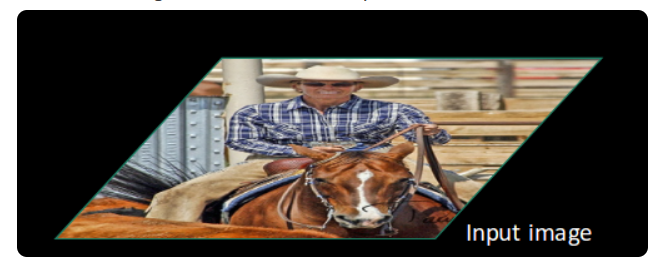
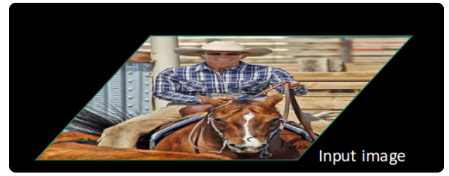
First, an image is taken as an input:
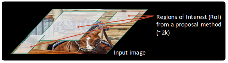
Then, we get the Regions of Interest (ROI) using some proposal method (for example, selective search as seen above):
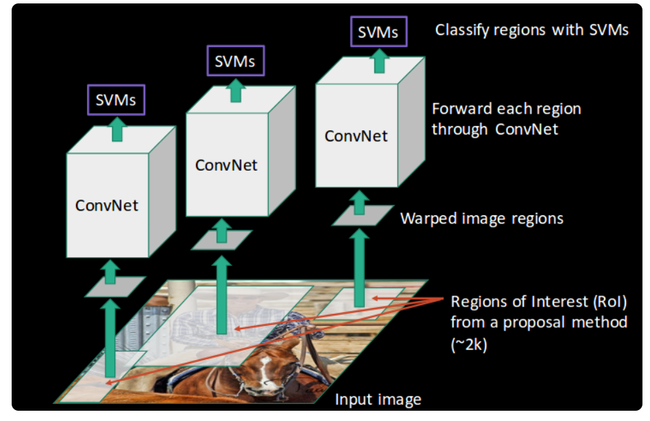
All these regions are then reshaped as per the input of the CNN, and each region is passed to the ConvNet:

CNN then extracts features for each region and SVMs are used to divide these regions into different classes:
Finally, a bounding box regression (Bbox reg) is used to predict the bounding boxes for each identified region:
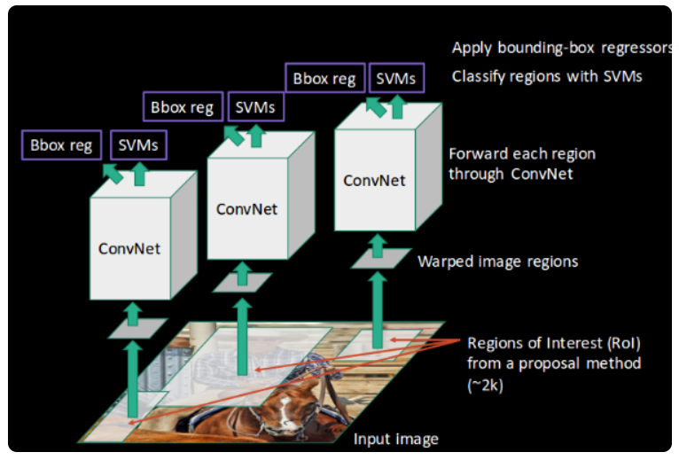
And this, in a nutshell, is how an RCNN helps us to detect objects.
Limitations of RCNN
Training an RCNN model is expensive and slow:
- Extracting 2,000 regions for each image based on selective search
- Extracting features using CNN for every image region. Suppose we have N images, then the number of CNN features will be N*2,000
- The entire process of object detection using RCNN has three models:
- CNN for feature extraction
- Linear SVM classifier for identifying objects
- Regression model for tightening the bounding boxes.
All these processes combine to make RCNN very slow. It takes around 40-50 seconds to make predictions for each new image, which essentially makes the model cumbersome and practically impossible to build when faced with a gigantic dataset.
Here’s the good news – we have another object detection technique which fixes most of the limitations we saw in RCNN.
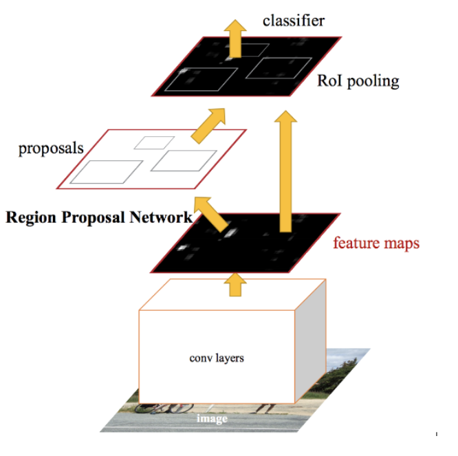
10.1.2 Understanding Fast RCNN
Intuition of Fast RCNN
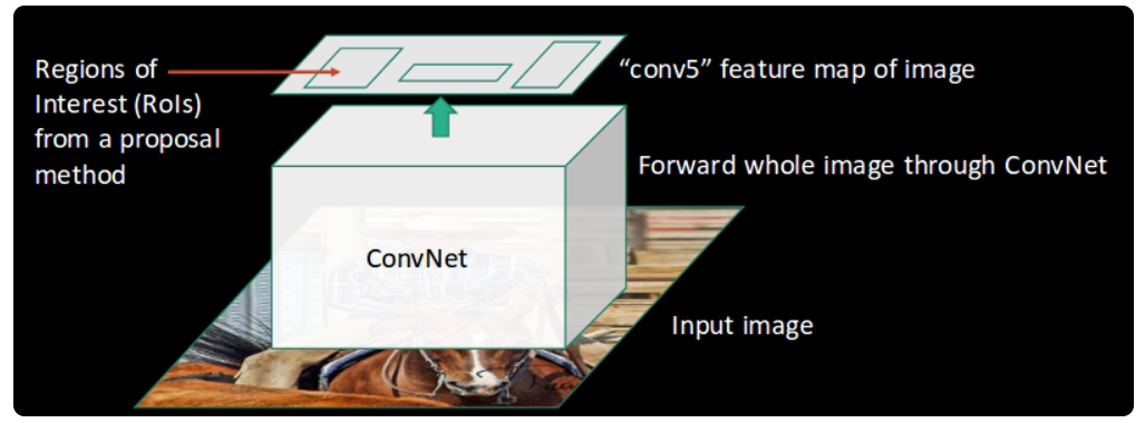
What else can we do to reduce the computation time a RCNN algorithm typically takes? Instead of running a CNN 2,000 times per image, we can run it just once per image and get all the regions of interest (regions containing some object).
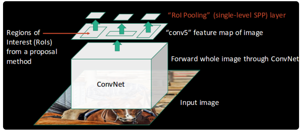
In Fast RCNN, we feed the input image to the CNN, which in turn generates the convolutional feature maps. Using these maps, the regions of proposals are extracted. We then use a RoI pooling layer to reshape all the proposed regions into a fixed size, so that it can be fed into a fully connected network.
Let’s break this down into steps to simplify the concept:
- As with the earlier two techniques, we take an image as an input.
- This image is passed to a ConvNet which in turns generates the Regions of Interest.
- A RoI pooling layer is applied on all of these regions to reshape them as per the input of the ConvNet. Then, each region is passed on to a fully connected network.
- A softmax layer is used on top of the fully connected network to output classes. Along with the softmax layer, a linear regression layer is also used parallely to output bounding box coordinates for predicted classes.
So, instead of using three different models (like in RCNN), Fast RCNN uses a single model which extracts features from the regions, divides them into different classes, and returns the boundary boxes for the identified classes simultaneously.
图解:
Taking an image as input:
This image is passed to a ConvNet which returns the region of interests accordingly:
Then we apply the RoI pooling layer on the extracted regions of interest to make sure all the regions are of the same size:
Finally, these regions are passed on to a fully connected network which classifies them, as well as returns the bounding boxes using softmax and linear regression layers simultaneously:
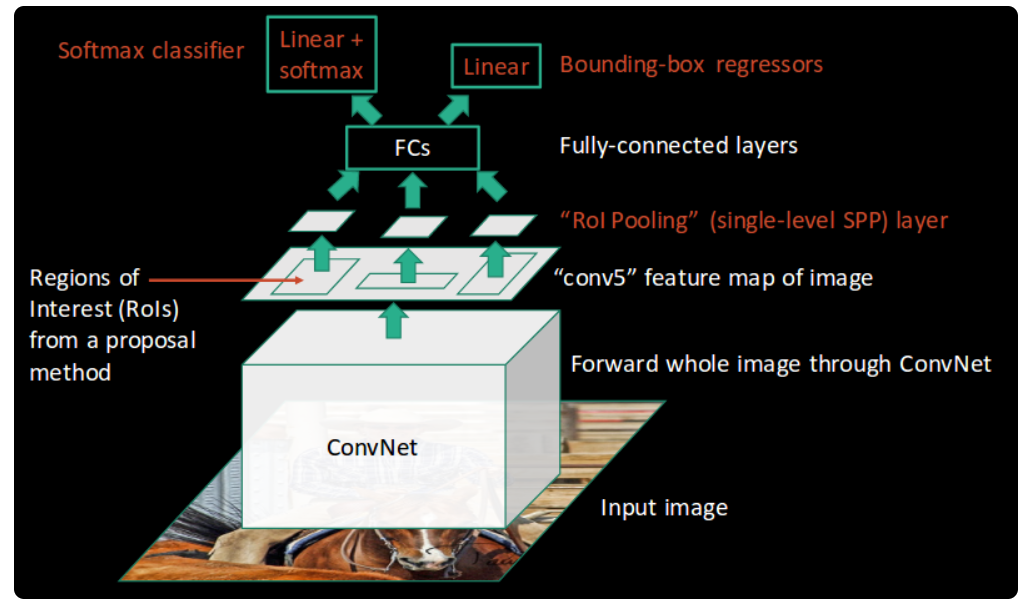
This is how Fast RCNN resolves two major issues of RCNN, i.e., passing one instead of 2,000 regions per image to the ConvNet, and using one instead of three different models for extracting features, classification and generating bounding boxes.
Limitations of Fast RCNN
It also uses selective search as a proposal method to find the Regions of Interest, which is a slow and time consuming process. It takes around 2 seconds per image to detect objects, which is much better compared to RCNN. But when we consider large real-life datasets, then even a Fast RCNN doesn’t look so fast anymore.
But there’s yet another object detection algorithm that trump Fast RCNN.
10.1.3 Understanding Faster RCNN
Intuition of Faster RCNN
Faster RCNN is the modified version of Fast RCNN. The major difference between them is that Fast RCNN uses selective search for generating Regions of Interest, while Faster RCNN uses “Region Proposal Network”, aka RPN. RPN takes image feature maps as an input and generates a set of object proposals, each with an objectness score as output.
The below steps are typically followed in a Faster RCNN approach:
- We take an image as input and pass it to the ConvNet which returns the feature map for that image.
- Region proposal network is applied on these feature maps. This returns the object proposals along with their objectness score.
- A RoI pooling layer is applied on these proposals to bring down all the proposals to the same size.
- Finally, the proposals are passed to a fully connected layer which has a softmax layer and a linear regression layer at its top, to classify and output the bounding boxes for objects.
A briefly explain how this Region Proposal Network (RPN) actually works.
Limitations of Faster RCNN
All of the object detection algorithms we have discussed so far use regions to identify the objects. The network does not look at the complete image in one go, but focuses on parts of the image sequentially. This creates two complications:
- The algorithm requires many passes through a single image to extract all the objects
- As there are different systems working one after the other, the performance of the systems further ahead depends on how the previous systems performed
10.1.4 Summary
| Algorithm | Features | Prediction time / image | Limitations |
|---|---|---|---|
| CNN | Divides the image into multiple regions and then classify each region into various classes. | – | Needs a lot of regions to predict accurately and hence high computation time. |
| RCNN | Uses selective search to generate regions. Extracts around 2000 regions from each image. | 40-50 seconds | High computation time as each region is passed to the CNN separately also it uses three different model for making predictions. |
| Fast RCNN | Each image is passed only once to the CNN and feature maps are extracted. Selective search is used on these maps to generate predictions. Combines all the three models used in RCNN together. | 2 seconds | Selective search is slow and hence computation time is still high. |
| Faster RCNN | Replaces the selective search method with region proposal network which made the algorithm much faster. | 0.2 seconds | Object proposal takes time and as there are different systems working one after the other, the performance of systems depends on how the previous system has performed. |
10.2 Implementing Faster RCNN for Object Detection (代码)
10.3 Object Detection using YOLO (含代码)
The R-CNN family of techniques we saw in Part 1 primarily use regions to localize the objects within the image. The network does not look at the entire image, only at the parts of the images which have a higher chance of containing an object.
The YOLO framework (You Only Look Once) on the other hand, deals with object detection in a different way. It takes the entire image in a single instance and predicts the bounding box coordinates and class probabilities for these boxes. The biggest advantage of using YOLO is its superb speed – it’s incredibly fast and can process 45 frames per second. YOLO also understands generalized object representation.
YOLO is a state-of-the-art object detection algorithm that is incredibly fast and accurate
Training
The input for training our model will obviously be images and their corresponding y labels. Let’s see an image and make its y label:
Consider the scenario where we are using a 3 x 3 grid with two anchors per grid, and there are 3 different object classes. So the corresponding y labels will have a shape of 3 x 3 x 16. Now, suppose if we use 5 anchor boxes per grid and the number of classes has been increased to 5. So the target will be 3 x 3 x 10 x 5 = 3 x 3 x 50. This is how the training process is done – taking an image of a particular shape and mapping it with a 3 x 3 x 16 target (this may change as per the grid size, number of anchor boxes and the number of classes).
Testing
The new image will be divided into the same number of grids which we have chosen during the training period. For each grid, the model will predict an output of shape 3 x 3 x 16 (assuming this is the shape of the target during training time). The 16 values in this prediction will be in the same format as that of the training label. The first 8 values will correspond to anchor box 1, where the first value will be the probability of an object in that grid. Values 2-5 will be the bounding box coordinates for that object, and the last three values will tell us which class the object belongs to. The next 8 values will be for anchor box 2 and in the same format, i.e., first the probability, then the bounding box coordinates, and finally the classes.
Finally, the Non-Max Suppression technique will be applied on the predicted boxes to obtain a single prediction per object.
That brings us to the end of the theoretical aspect of understanding how the YOLO algorithm works, starting from training the model and then generating prediction boxes for the objects. Below are the exact dimensions and steps that the YOLO algorithm follows:
- Takes an input image of shape (608, 608, 3)
- Passes this image to a convolutional neural network (CNN), which returns a (19, 19, 5, 85) dimensional output
- The last two dimensions of the above output are flattened to get an
output volume of (19, 19, 425):
- Here, each cell of a 19 X 19 grid returns 425 numbers
- 425 = 5 * 85, where 5 is the number of anchor boxes per grid
- 85 = 5 + 80, where 5 is (pc, bx, by, bh, bw) and 80 is the number of classes we want to detect
- Finally, we do the IoU and Non-Max Suppression to avoid selecting overlapping boxes
10.4 Object detection by Stanford
10.5 其他Resources
11. Project 3 - Face Counting Challenge
12. Project 4 - COCO Object Detection Challenge
http://cocodataset.org/#download
13. Image Segmentation
13.1 A Step-by-Step Introduction to Image Segmentation Techniques
13.1.1 What is Image Segmentation?
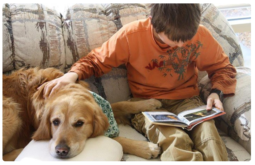
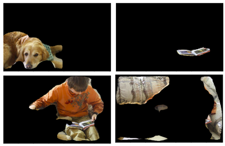
An image is a collection or set of different pixels. We group together the pixels that have similar attributes using image segmentation. Take a moment to go through the below visual (it’ll give you a practical idea of image segmentation):
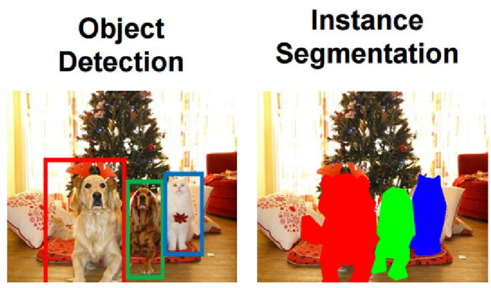
Object detection builds a bounding box corresponding to each class in the image. But it tells us nothing about the shape of the object. We only get the set of bounding box coordinates. We want to get more information – this is too vague for our purposes.
Image segmentation creates a pixel-wise mask for each object in the image. This technique gives us a far more granular understanding of the object(s) in the image.
13.1.2 Why do we need Image Segmentation?
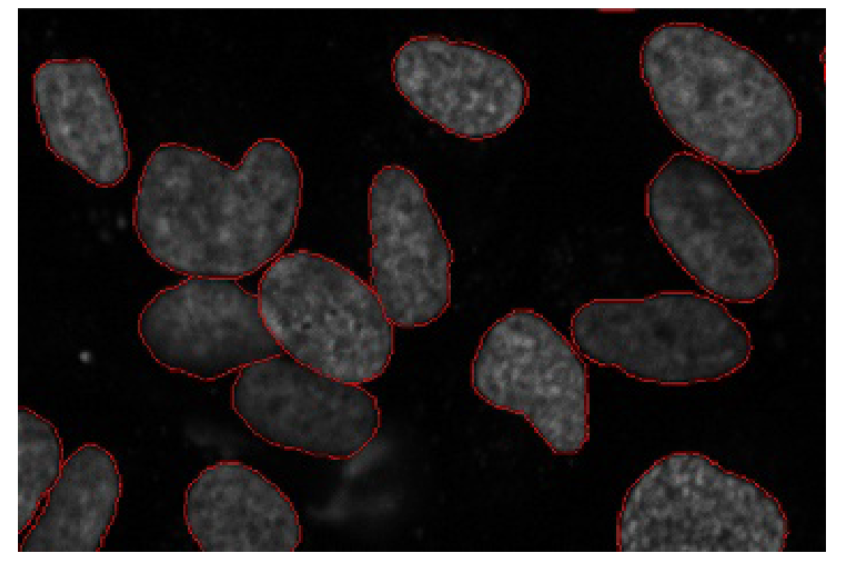
Cancer has long been a deadly illness. Even in today’s age of technological advancements, cancer can be fatal if we don’t identify it at an early stage. Detecting cancerous cell(s) as quickly as possible can potentially save millions of lives.
The shape of the cancerous cells plays a vital role in determining the severity of the cancer. You might have put the pieces together – object detection will not be very useful here. We will only generate bounding boxes which will not help us in identifying the shape of the cells.
Image Segmentation techniques make a MASSIVE impact here. They help us approach this problem in a more granular manner and get more meaningful results. A win-win for everyone in the healthcare industry.
There are many other applications where Image segmentation is transforming industries:
- Traffic Control Systems
- Self Driving Cars
- Locating objects in satellite images
13.1.3 The Different Types of Image Segmentation
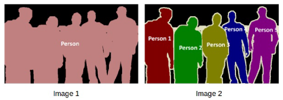
If there are 5 people in an image, semantic segmentation will focus on classifying all the people as a single instance. Instance segmentation, on the other hand. will identify each of these people individually.
13.1.4 Region-based Segmentation (Threshold)
One simple way to segment different objects could be to use their pixel values. An important point to note – the pixel values will be different for the objects and the image’s background if there’s a sharp contrast between them.
In this case, we can set a threshold value. The pixel values falling below or above that threshold can be classified accordingly (as an object or the background). This technique is known as Threshold Segmentation.
If we want to divide the image into two regions (object and background), we define a single threshold value. This is known as the global threshold.
If we have multiple objects along with the background, we must define multiple thresholds. These thresholds are collectively known as the local threshold.
代码见这里.
You can set different threshold values and check how the segments are made. Some of the advantages of this method are:
- Calculations are simpler
- Fast operation speed
- When the object and background have high contrast, this method performs really well
But there are some limitations to this approach. When we don’t have significant grayscale difference, or there is an overlap of the grayscale pixel values, it becomes very difficult to get accurate segments.
13.1.5 Edge Detection Segmentation
What divides two objects in an image? There is always an edge between two adjacent regions with different grayscale values (pixel values). The edges can be considered as the discontinuous local features of an image.
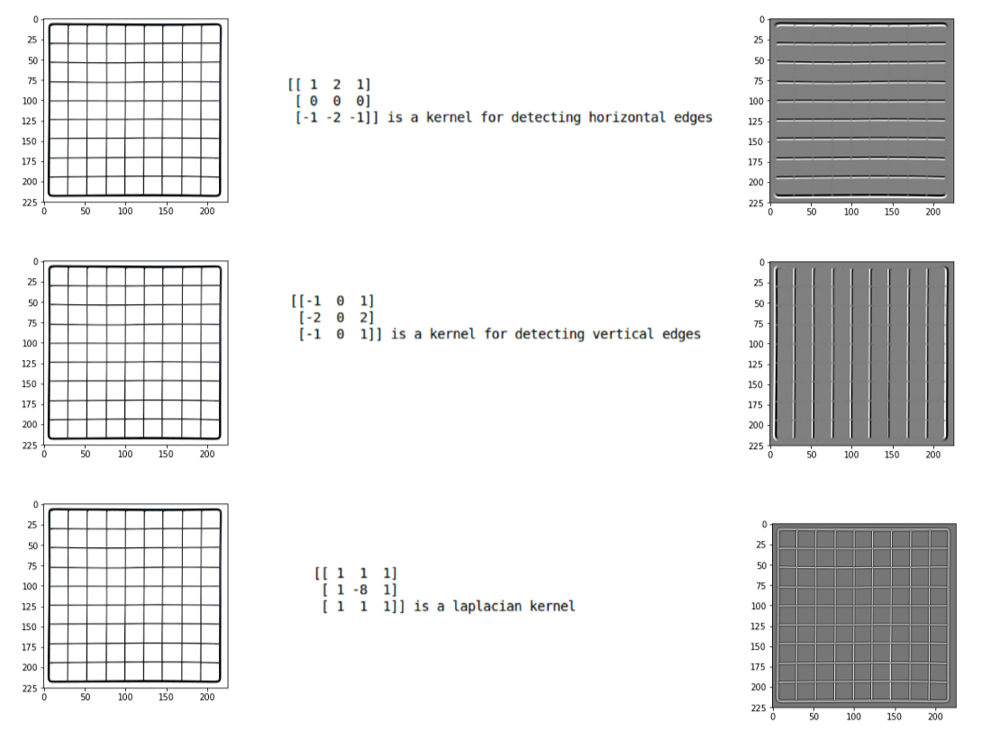
We can make use of this discontinuity to detect edges and hence define a boundary of the object. This helps us in detecting the shapes of multiple objects present in a given image. Now the question is how can we detect these edges? This is where we can make use of filters and convolutions. Refer to this article if you need to learn about these concepts.
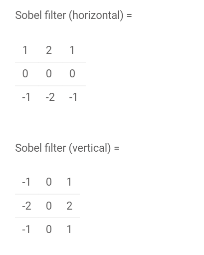
Researchers have found that choosing some specific values for these weight matrices (filters) helps us to detect horizontal or vertical edges (or even the combination of horizontal and vertical edges).
One such weight matrix is the sobel operator. It is typically used to detect edges.
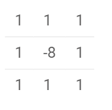
There is one more type of filter that can detect both horizontal and vertical edges at the same time. This is called the laplace operator:
例:
代码见这里.
13.1.6 Image Segmentation based on Clustering
Clustering is the task of dividing the population (data points) into a number of groups, such that data points in the same groups are more similar to other data points in that same group than those in other groups. These groups are known as clusters.
One of the most commonly used clustering algorithms is k-means. Here, the k represents the number of clusters (not to be confused with k-nearest neighbor). Let’s understand how k-means works:
- First, randomly select k initial clusters
- Randomly assign each data point to any one of the k clusters
- Calculate the centers of these clusters
- Calculate the distance of all the points from the center of each cluster
- Depending on this distance, the points are reassigned to the nearest cluster
- Calculate the center of the newly formed clusters
- Finally, repeat steps (4), (5) and (6) until either the center of the clusters does not change or we reach the set number of iterations
The key advantage of using k-means algorithm is that it is simple and easy to understand. We are assigning the points to the clusters which are closest to them.
代码见这里.
选择5 cluster的效果:
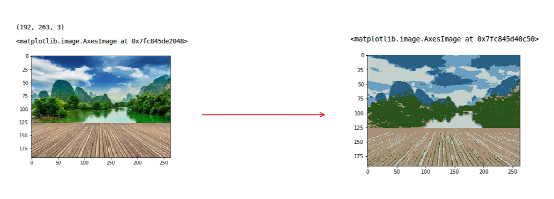
k-means works really well when we have a small dataset. It can segment the objects in the image and give impressive results. But the algorithm hits a roadblock when applied on a large dataset (more number of images).
It looks at all the samples at every iteration, so the time taken is too high. Hence, it’s also too expensive to implement. And since k-means is a distance-based algorithm, it is only applicable to convex datasets and is not suitable for clustering non-convex clusters.
Finally, let’s look at a simple, flexible and general approach for image segmentation.
13.1.7 Mask R-CNN
Mask R-CNN is an extension of the popular Faster R-CNN object detection architecture. Mask R-CNN adds a branch to the already existing Faster R-CNN outputs. The Faster R-CNN method generates two things for each object in the image:
- Its class
- The bounding box coordinates
Mask R-CNN adds a third branch to this which outputs the object mask as well. Take a look at the below image to get an intuition of how Mask R-CNN works on the inside:
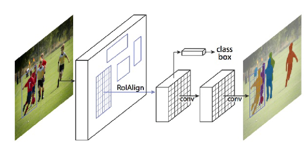
- We take an image as input and pass it to the ConvNet, which returns the feature map for that image
- Region proposal network (RPN) is applied on these feature maps. This returns the object proposals along with their objectness score
- A RoI pooling layer is applied on these proposals to bring down all the proposals to the same size
- Finally, the proposals are passed to a fully connected layer to classify and output the bounding boxes for objects. It also returns the mask for each proposal
Mask R-CNN is the current state-of-the-art for image segmentation and runs at 5 fps.
13.1.8 Summary
| Algorithm | Description | Advantages | Limitations |
|---|---|---|---|
| Region-Based Segmentation | Separates the objects into different regions based on some threshold value(s). | a. Simple calculationsb. Fast operation speedc. When the object and background have high contrast, this method performs really well | When there is no significant grayscale difference or an overlap of the grayscale pixel values, it becomes very difficult to get accurate segments. |
| Edge Detection Segmentation | Makes use of discontinuous local features of an image to detect edges and hence define a boundary of the object. | It is good for images having better contrast between objects. | Not suitable when there are too many edges in the image and if there is less contrast between objects. |
| Segmentation based on Clustering | Divides the pixels of the image into homogeneous clusters. | Works really well on small datasets and generates excellent clusters. | a. Computation time is too large and expensive.b. k-means is a distance-based algorithm. It is not suitable for clustering non-convex clusters. |
| Mask R-CNN | Gives three outputs for each object in the image: its class, bounding box coordinates, and object mask | a. Simple, flexible and general approachb. It is also the current state-of-the-art for image segmentation | High training time |
13.2 Implementing Mask R-CNN for Image Segmentation
13.2.1 Understanding Mask R-CNN
Mask R-CNN is basically an extension of Faster R-CNN. Faster R-CNN is widely used for object detection tasks. For a given image, it returns the class label and bounding box coordinates for each object in the image.
The Mask R-CNN framework is built on top of Faster R-CNN. So, for a given image, Mask R-CNN, in addition to the class label and bounding box coordinates for each object, will also return the object mask.
Let’s first quickly understand how Faster R-CNN works. This will help us grasp the intuition behind Mask R-CNN as well.
- Faster R-CNN first uses a ConvNet to extract feature maps from the images
- These feature maps are then passed through a Region Proposal Network (RPN) which returns the candidate bounding boxes
- We then apply an RoI pooling layer on these candidate bounding boxes to bring all the candidates to the same size
- And finally, the proposals are passed to a fully connected layer to classify and output the bounding boxes for objects
Once you understand how Faster R-CNN works, understanding Mask R-CNN will be very easy. So, let’s understand it step-by-step starting from the input to predicting the class label, bounding box, and object mask.
第一步:Backbone Model
Similar to the ConvNet that we use in Faster R-CNN to extract feature maps from the image, we use the ResNet 101 architecture to extract features from the images in Mask R-CNN. So, the first step is to take an image and extract features using the ResNet 101 architecture. These features act as an input for the next layer.
第二步:Region Proposal Network (RPN)
Now, we take the feature maps obtained in the previous step and apply a region proposal network (RPM). This basically predicts if an object is present in that region (or not). In this step, we get those regions or feature maps which the model predicts contain some object.
第三步:Region of Interest (RoI)
The regions obtained from the RPN might be of different shapes, hence, we apply a pooling layer and convert all the regions to the same shape. Next, these regions are passed through a fully connected network so that the class label and bounding boxes are predicted.
Till this point, the steps are almost similar to how Faster R-CNN works. Now comes the difference between the two frameworks. In addition to this, Mask R-CNN also generates the segmentation mask.
For that, we first compute the region of interest so that the computation time can be reduced. For all the predicted regions, we compute the Intersection over Union (IoU) with the ground truth boxes. We can computer IoU like this:
IoU = Area of the intersection / Area of the union
Now, only if the IoU is greater than or equal to 0.5, we consider that as a region of interest. Otherwise, we neglect that particular region. We do this for all the regions and then select only a set of regions for which the IoU is greater than 0.5.
Let’s understand it using an example. Consider this image:
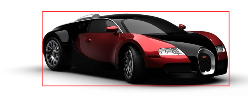
Here, the red box is the ground truth box for this image. Now, let’s say we got 4 regions from the RPN as shown below:
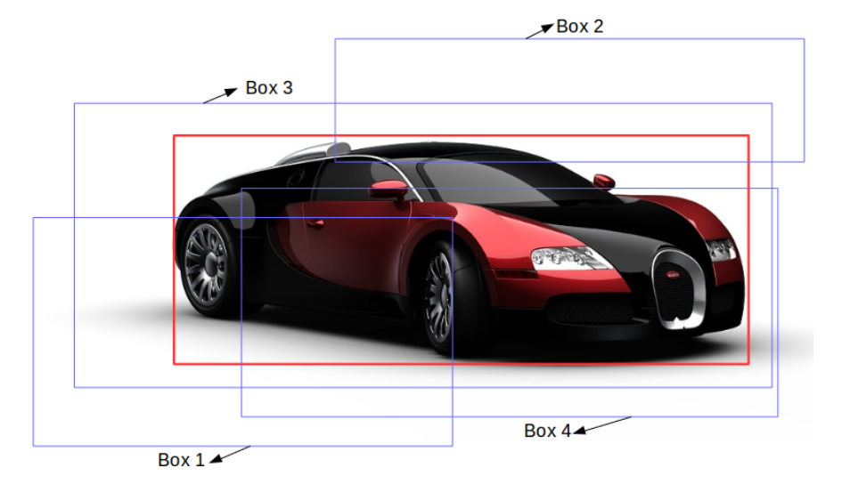
Here, the IoU of Box 1 and Box 2 is possibly less than 0.5, whereas the IoU of Box 3 and Box 4 is approximately greater than 0.5. Hence. we can say that Box 3 and Box 4 are the region of interest for this particular image whereas Box 1 and Box 2 will be neglected.
Next, let’s see the final step of Mask R-CNN.
第四步:Segmentation Mask
Once we have the RoIs based on the IoU values, we can add a mask branch to the existing architecture. This returns the segmentation mask for each region that contains an object. It returns a mask of size 28 X 28 for each region which is then scaled up for inference.
Again, let’s understand this visually. Consider the following image:
The segmentation mask for this image would look something like this:
Here, our model has segmented all the objects in the image. This is the final step in Mask R-CNN where we predict the masks for all the objects in the image.
Keep in mind that the training time for Mask R-CNN is quite high. It took me somewhere around 1 to 2 days to train the Mask R-CNN on the famous COCO dataset. So, for the scope of this article, we will not be training our own Mask R-CNN model.
We will instead use the pretrained weights of the Mask R-CNN model trained on the COCO dataset. We will be using the mask rcnn framework created by the Data scientists and researchers at Facebook AI Research (FAIR).
13.2.2 Implement Mask R-CNN
代码见这里.