Excel中的常见操作

1.筛选后求和、求平均值

参考：subtotal函数，SUBTOTAL function - Microsoft Support

在经过筛选后，如果使用sum()函数进行求和，选择的其实包含了被筛选掉的列。也即选中时并没有选中筛选后的列，这样求出来的和不是想要的。注：在选中筛选的内容后，excel右下角的求和是正确的。

改用subtotal函数：

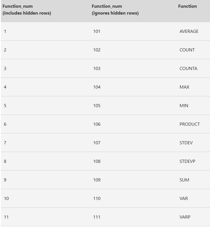
SUBTOTAL(function_num,ref1,[ref2],...)

求和：

SUBTOTAL(109,选中列)

求均值：

SUBTOTAL(101,选中列)

Function_num Required. The number 1-11 or 101-111 that specifies the function to use for the subtotal. 1-11 includes manually-hidden rows, while 101-111 excludes them; filtered-out cells are always excluded. （1-11包含了hidden rows，101-111剔除了filtered-out cells）

注：且筛选内容变了后，对应的结果也会跟着变，不用把函数删掉再重写。

2. vlookup 与 xlookup

参考：Beginner’s Guide to XLOOKUP vs VLOOKUP in Excel | Zero To Mastery

Both VLOOKUP and XLOOKUP are made for a single task - finding information in a table.

You’re telling Excel,

“Find this thing, then give me the matching value.”

Both VLOOKUP and XLOOKUP do the same job. The difference is how they do it, and how much control they give you. That’s where things start to get interesting.

VLOOKUP: The name stands for “vertical lookup,” and that’s exactly what it does: it searches down the first column of a table to find a match, then returns a value from another column in the same row.

例如：Let’s say you have a table with product IDs in column A and prices in column B. If you want to look up the price for product ID 123 in that table, you’d write:

=VLOOKUP(123, A:B, 2, FALSE)
或写成：
=VLOOKUP(123, A:B, 2, 0)

缺点：

• The first issue is that the column number is hard-coded. If you add or remove columns later, the formula might break or pull the wrong value （要数第几列是想返回的）
• Not only that but VLOOKUP only searches from left to right. If your return value is in a column to the left of what you’re searching, it won’t work （搜索是从左到右的，要查找的列得在第一列，返回列得在查找列的右边）
• And finally, if you forget to include FALSE at the end, Excel will try to return an approximate match instead of an exact one. That can lead to subtle, frustrating errors

新版本的excel引入了XLOOKUP (If you’re using Excel 2016 or earlier, XLOOKUP won’t work. It was introduced in Excel 365 and Excel 2019, so older versions won’t recognize the function at all.)

At its core, XLOOKUP is still about matching a value and returning related data. But XLOOKUP formulas are easier to read, easier to write, and a lot less fragile.

还是之前的例子，用XLOOKUP来写：

=XLOOKUP(123, A:A, B:B)

Instead of counting columns, you tell Excel exactly where to look and exactly where to return the value from. A:A is your lookup range. B:B is your return range. （A:A代表查找的范围，B:B代表返回的范围，并且还支持返回多列，例如B:C则会返回B,C两列的内容）

That’s it. There’s no need to worry about moving columns around, OR fetching values from the wrong column because you miscounted by one or two (which, believe me, is surprisingly easy to do!).

You can also search from right to left, something VLOOKUP can’t do. And by default, XLOOKUP looks for an exact match, so you don’t need that extra TRUE/FALSE argument at the end of the formula.

Oh, and it also has built-in error handling!

For example:

=XLOOKUP(123, A:A, B:B, "Not found")

If Excel doesn’t find a match, it returns the message “Not found” instead of showing an error like #N/A.

2.1 vlookup根据两列数据匹配

参考 https://zhuanlan.zhihu.com/p/68744986

当两列数据确定唯一值时，例如：有数据：

季度	客户经理	接待人数	开户数
21Q1	A	xx	？
21Q2	A	xx
21Q3	A	xx
21Q1	B	xx
21Q2	B	xx
21Q3	B	xx

此时想根据季度与客户经理去匹配另一张表中的开户数时，有如下方法：

=VLOOKUP(E2&F2,IF({1,0},A1:A13&B1:B13,C1:C13),2,FALSE)

↑在开户数这一列，写入上面的公式，再双击填充。其中E2与F2指季度与客户经理这两列(单元格)，A1:A13与B1:B13指有开户数的那张表中的季度与客户经理两列（用&拼接起来），C1:C13为开户数那一列。

IF({1,0},A1:A13&B1:B13,C1:C13) 的含义：
IF(条件,返回值1,返回值2)，如果条件为真，返回"返回值1"，如果条件为假，返回"返回值2"。
{1,0}，则代表选择一个数组，第一列为真，即第一列返回"返回值1"，A1:A13&B1:B13，第二列为假，即第二列返回"返回值2"，C1:C13

可以认为IF({1,0})的写法是为了选取不连续的列(拼接后的数组看成一列，并再选中其他列)放到一个参数中

倒数第二个参数2代表C1:C13开户数这列，位于选取的范围中的第2列（A1:A13&B1:B13视为第1列）

2.2 xlookup根据两列数据匹配

=xlookup(E2&F2,A:A&B:B,C:C,"")  # 如果没有匹配的返回空

3.countif函数

参考 Excel函数公式：关于Countif函数的用法，你知道多少？

countif(range, criteria)

示例1：

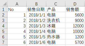
计算电脑的销售数量：

=COUNTIF(C2:C7,"电脑")

另：可结合通配符使用。例如统计包含”电脑“的销售数量：

=COUNTIF(C2:C7,"*电脑*")

示例2：

指定条件计数，例如统计销售额大于平均金额的个数：

=COUNTIF(D2:D7,">"&AVERAGE(D2:D7))

条件用到了另外的一个函数，我们需要用符号“&”来作为连接符号。否则无法得到正确的结果。

4.sumif函数

参考 Excel函数公式：条件求和：SUMIF函数！！！

SUMIF(range,criteria,[sum_range])

range:用于条件计算的单元格
criteria:用于确定对求和单元格的田间
sum_range:要求和的实际单元格。如果省略sum_range参数，Excel会对在range参数中指定的单元格（即应用条件的单元格）求和。

示例1：

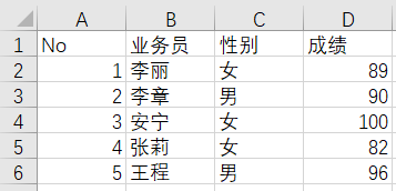
求女生成绩之和：

=SUMIF(C2:D6,"女",D2:D6)
也可写作
=SUMIF(C2:C6,"女",D2:D6)

示例2：

大于89的成绩之和：

=SUMIF(D2:D6,">89")

示例3：

李丽，李章，王程成绩之和：

=SUM(SUMIF(B2:B6,{"李丽","李章","王程"},D2:D6))

示例4：

求前3名成绩之和：

=SUMIF(D2:D6,">="&LARGE(D2:D6,3))

函数LARGE(RANGE,K)的作用是返回数组中第K个最大值

↑注：如果有两个第3大的值，large(range,3) 与 large(range,4) 会返回一样的值。